Abstract
Objectives During the early stage of COVID-19 spread, many governments and regional jurisdictions put in place travel restrictions and imposed quarantine after arrivals in an effort to slow down or stop the importation of cases. At the same time, they implemented non-pharmaceutical interventions (NPI) to curtail local spread. We assess the risk of importation of COVID-19 in locations that are at that point without infection or where local chains of transmission have extinguished, and evaluate the role of quarantine in this risk.
Methods A stochastic SLIAR epidemic model is used. The effect of the rate, size, and nature of importations is studied and compared to that of NPI on the risk of importation-induced local transmission chains. The effect of quarantine on the rate of importations is assessed, as well as its efficacy as a function of its duration.
Results The rate of importations plays a critical role in determining the risk that case importations lead to local transmission chains, more so than local transmission characteristics, i.e., strength of NPI. The latter influences the severity of the outbreaks. Quarantine after arrival in a location is an efficacious way to reduce the rate of importations.
Conclusions Locations that see no or low level local transmission should ensure that the rate of importations remains low. A high level of compliance with post-arrival quarantine followed by testing achieves this objective with less of an impact than travel restrictions or bans.
1 Introduction
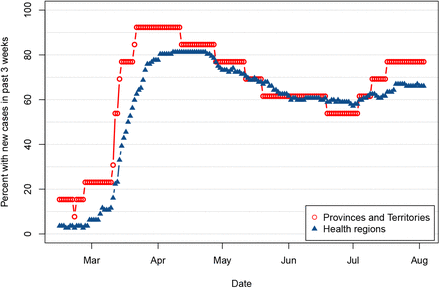
The spatio-temporal spread of COVID-19 is documented by a sequence of importation times reported at different administrative levels. See, for instance, the works1–4 for accounts of early post-importation spread in several countries. Canada is used here as an example; the first confirmed case was reported in Ontario on 25 January 2020. British Columbia reported a case on 28 January 2020, but other provinces and territories (P/T) did not report cases until March or later, with Nunavut still having not reported confirmed cases at the time of writing. Figure 1 shows the evolution of the percentage of jurisdictions having reported at least one new case in the past three weeks, for P/T and 112 Canadian health regions.5, 6 The initial increase in the number of jurisdictions affected was entirely driven by case importations to these jurisdictions. Later increases are indicative of importation of a case from another jurisdiction or existence of silent transmission chains lasting more than three weeks.
Percentage of provinces, territories and health regions in Canada having declared new confirmed cases of COVID-19 in 2020 in a three weeks period.
In the first phase of the pandemic, most countries (or lower level bodies in federal countries with devolved health care) took global, one-size-fits-all measures. After this initial lockdown period during which travel was also severely hampered, a second phase has now started, with local transmission down in some jurisdictions. However, with no therapeutic tools or vaccines yet available, preparations must be made for a potential increase of transmission in some jurisdictions. Were this to happen, many locations would be re-importing cases. It seems important, in this context, to apply a more measured approach than the total top jurisdiction-level lockdowns that were used; the enormous economic cost of the first wave of lockdowns, combined with the potential diminishing compliance of individuals with public health measures, impose that public health authorities find ways to mitigate spread that are finer grained.
As part of the arsenal of measures available to public health authorities in the fight against the spread of COVID-19, there are some that are specifically geared towards the reduction of the risk of case importations: travel restrictions or bans, self-isolation upon arrival, etc. See the Electronic Supplement A.1 for details These measures have different effects and varying efficacy. In order to evaluate their relative effectiveness, it is important to better understand the importation process.
Some works7–16 have considered the link between transportation and importation of COVID-19. We complement these works here by finely decomposing the process through which cases are imported into different types of events and focusing on the role of the rate at which a location is “challenged” by importations. We also consider the efficacy of the main method for reducing this rate while maintaining mobility: quarantine.
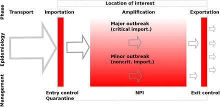
Importations are a critical component in the spatialisation of COVID-19 and other emerging or re-emerging infectious diseases, the overall spread phenomenon being driven by the repetition of transport, importation, amplification and exportation events. We further classify importations as unsuccessful if they do not lead to any local transmission chains or successful if they do. Successful importations then depend on the type of transmission chains they generate: they are noncritical or critical if they lead, respectively, to minor or major outbreaks. See Figure 2 and A.1 for details.
Spatialisation process: transport of cases from other locations; importation into the location of interest; local amplification; exportation to other locations. Red indicates control methods. See A.1 for details.
Here, we consider importations of COVID-19 to locations that are not in the amplification stage and where importations could tip the balance in the direction of entering amplification. These include locations that have not had local cases yet, saw local transmission chains that have since extinguished or are seeing limited local transmission. The main issue tackled in this paper is the assessment of the risk that a successful importation occurs depending on the rate of case importations and local conditions, as well as the effect of post-arrival quarantine on these rates. To consider the problem, we use an SLIAR model “stimulated” by individuals flowing in from other locations.
2 Methods
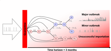
To track individual events and gain access to quantities such as the proportion of successful importations, we formulate the model as a continuous time Markov chain (CTMC).17 The setting under consideration is a single location in which the population is assumed to be homogeneously mixing. Initially, there are no active cases in the community; the model tracks the fate of the cohort of individuals who are susceptible to the disease. We consider the short term response of the model to stimulations taking the form of inflow of infected individuals, as schematised in Figure 3.
Input-output setting: imports arrive through transport, are potentially funnelled through quarantine, then enter one of the infected compartments. The three types of outcomes considered are shown on the right.
2.1 Epidemiological model and parameters
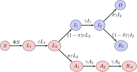
The structure of the model is detailed in A.2 and A.3, with the epidemiological model detailed in Figure ES.8: susceptible individuals, upon infection, move to the latent compartment. (Incubation and latent periods are assumed to overlap.) When their latent period is over, they can either progress to a symptomatic infection or to an asymptomatic one. At the end of the infectious period, individuals are removed (they recover or die); they no longer spread the disease. Post-recovery immunity is assumed to last at least as long as the (short) period of time under consideration.
We adopt a case detection-based approach. Symptomatically infectious individuals are those who have been detected through testing, reporting or hospitalisation, i.e., individuals who appear as confirmed cases in the data. Asymptomatically infectious individuals include those who are asymptomatic in the usual sense, but also symptomatic cases that avoid detection because of lack of testing. In the perspective of response to a crisis, using such a case detection-based definition for symptomatic and asymptomatic individuals allows to tailor model outputs to the situation in the location under consideration. This is further enhanced by using compartments RI and D directly connected to published data (Figures 3 and ES.8). One drawback from using a case detection-based distinction between symptomatic and asymptomatic cases is that the parameters involved (π, δ and η) incorporate not only disease characteristics but also some information about health policies specific to the location under consideration. For instance, locations performing a lot of testing have a lower proportion of individuals following the asymptomatic route, i.e., a lower value of π, than those doing less testing.
Model parameters.
Simulations are tailored to locations, i.e., health regions or cities. The initial susceptible population, S(0), is the total population of the location under consideration, adjusted for pre-existing immunity if transmission occurred in the past. Epidemiological parameters are the means of those in18 as well as values commonly found in the literature. Epidemiological and importation parameters are listed in Table 1. Simulations are run using the exact method in the R package GillespieSSA2 with a time horizon of three months (92 days). Unless otherwise indicated, 1,000 simulations are run for each combination of parameter values and, when applicable, initial conditions.
2.2 Response of the system to case importations
Inputs to the system with transition probabilities (ES.3) are the importation events, i.e., stimulations taking the form of inflow of infected individuals as described by (ES.5); outputs are the responses of the system to these importation events. The nature of importation events and resulting outputs considered are summarised in Table 2.
Of particular interest here is the consideration of these responses in terms of the severity of importations as defined in A.1 and briefly summarised here.
An unsuccessful importation has the import case not resulting in the transmission of the disease to anyone in the local population; in other words, there are no susceptible to latent (S → L1) transitions.
A successful importation sees the import case resulting in at least one local case. Successful importations are further classified as follows.
A noncritical successful importation is one that is followed by a minor outbreak.
A critical successful importation is one followed by a major outbreak.
Minor and major outbreaks are defined as in a seminal paper of Whittle;19 see details in A.6. Finally, we say that the disease is locally extinct if there are no more cases of any type in the population under consideration.
3 Results
Table 2 summarises the questions investigated with the model and the outputs presented in the results.
3.1 Single stimulation simulations
3.1.1 Role of the type of importation
The nature of the import case is important, as evidenced in Table ES.3. As can be expected, the earlier in the disease cycle an infected individual is when they are introduced in a population, the longer they spend interacting with others and thus the higher the risk that they transmit the disease. For instance, from Table ES.3, importing a single L1 latent case is followed by a major outbreak in 11.5%  to 70.1%
  of simulations, while importation of an A1 asymptomatic case leads to a major outbreak in 3.5%
  to 30.2%
  of simulations. For comparison, a recent study by Kucharski et al15 found that a single importation leads to a large outbreak 17% to 25% of the time.
The nature of import cases is, to a large extent, a random hand that is dealt to importing jurisdictions. Unfortunately, most control measures they can implement “upstream” from an importation only have the capacity to remove symptomatically infectious individuals from the incoming flow, so that, in particular, latently infected individuals still can arrive.
3.1.2 Role of the size of the importation
The size of the importation is naturally a key factor in the risk of importation, as was already established by Kucharski et al.15 To illustrate this and using outbreak severity criteria defined in A.6, let us focus on importations of individuals in the L1 compartment. Qualitatively similar results are obtained by considering importations of other types of infected individuals but are not shown here.
Simulation strategies. Questions addressed with the model and specification of inputs and outputs used. Individuals of type  are those infected with the disease, i.e.,
  . Individuals of type
  are unobservable infected, i.e.,
  .
.
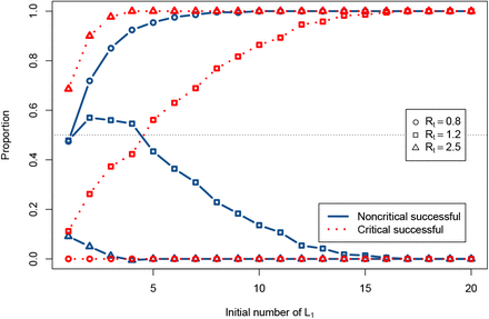
Figure 4 shows the proportion of simulations with successful importations followed by major and minor outbreaks as a function of the importation size, i.e., the initial number of L1 individuals, for different values of the effective reproduction number  . The proportion of simulations with critical successful importations, i.e., those followed by a major outbreak, is sensitive to the value of
  . Therefore, the value of
  may significantly change the outcome if several infected individuals arrive simultaneously. The proportion of simulations with noncritical successful importations shows a maximum at a given initial number of L1. Indeed, when the initial number of L1 increases, it is more likely to trigger a critical successful importation than a noncritical one.
Proportions of critical (dotted red) and noncritical successful (solid blue) importations as a function of the initial number of imported L1 cases. Circles:  , squares: 1.2 and triangles: 2.5.
Here, there are obvious implications in terms of disease control, since one of the mechanisms leading to multiple simultaneous importations is infection during transport. Take for instance a location maintaining good but not perfect local conditions  . If it receives four L1 individuals, then there is roughly a 50/50 chance that this leads to a major outbreak. If, on the other hand, these four individuals each infect another person during transport because of inadequate protocols aboard the incoming conveyance, then the odds of a major outbreak jump up to 3/4.
3.2 Effect of importation rates and NPI efficacy
We now consider the effect of repeated importations. We suppose that individuals arrive in the location through the importation process defined in (ES.5) by the Poisson distribution with parameter λ. The rate of importation λ from a given location can be approximated from epidemiological and travel characteristics of the origin location of the import case using (ES.6); the rate of importation from all sources is given in (ES.7). We vary 1/λ, the mean number of days between importation events. Here,  and
and  (we suppose I individuals are not able or allowed to travel).
Both the rate of case importations and the local effective reproduction number  have an effect on the capacity of the disease to become established in the population. The larger
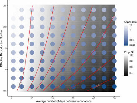
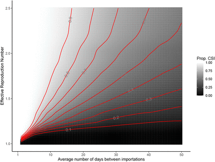
  , the less efficacious the NPI. The raster in Figure 5 shows the proportion of simulations with a successful importation over a three month period.
Proportion of successful importations (SI, grey scale) and attack rates (blue scale) in a 3 month period for different values of the average number of days 1/λ between two importations and  , an indicator of NPI efficacy.
When importations occur infrequently, local conditions are key. For instance, if importations occur on average every 40 days, local conditions change the risk of post-importation outbreaks over a three months period from roughly 40% to 70% of simulations. As the rate of case importations increases, post-importation outbreaks are increasingly likely for all local conditions, to the point that when cases are introduced every three days or less, 99% of simulations see outbreaks, regardless of the effort of local control. Thus, reducing the importation rate is key to preventing outbreaks.
On the other hand, the severity of the outbreaks is also sensitive to the value of  . The dots in Figure 5 show the attack rate of the disease in the population over the three months period considered, computed as the ratio (expressed as a percentage) (S(0)−S(tf))/S(0)), where S(0) and S(tf) are the number of susceptible individuals at the beginning and end of one simulation, respectively. Even though the probability of an outbreak is high when the rate of importations is high, regardless of local NPI effort, the intensity of local NPI effort greatly changes the outcome. Indeed, consider the attack rates where the average number of days between importations is one day (left-most column in Figure 5). Attack rates there range from 13.1% when
  to 0.02% when
  . So, although the probability of importing the disease is roughly equal for this high importation rate, the severity of outcomes is very different. For
  , we distinguish between minor and major outbreaks using the threshold τ defined in A.6. This is shown in Figure ES.10.
3.3 Effect of post-arrival quarantine
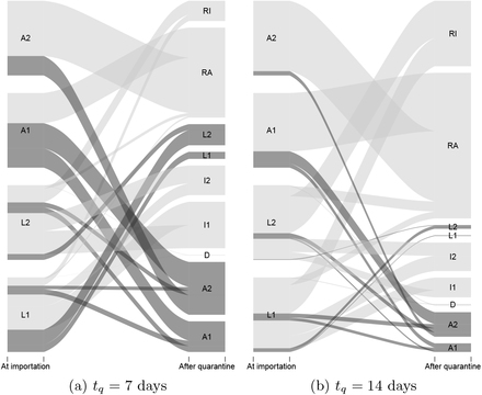
The rate of importations plays a critical role in the risk that importations will trigger local transmission chains (Figure 5). The status of individuals when they arrive is also very important (Table ES.3). In order to evaluate the benefit of post-arrival quarantine, we proceed to the following simple numerical experiment. We consider Poisson generated chains of importation events, where each importation event is one of L1, L2, A1 or A2, i.e., one of the undetected infected states. These chains are run through (ES.3) with no transmission (β = 0) and for tq days, where tq is the duration of quarantine. Running the chains with no transmission means we consider the evolution of each individual case through disease stages during the quarantine period. Figure 6 shows, for quarantine periods of 7 and 14 days, the transitions between stages at the beginning and end of quarantine. We highlight in dark grey individuals who are still a risk to the community at the end of their quarantine period since they are still in unobservable stages  (see B.6 for details).
Evolution of the status of import cases during a (left) one or (right) two week quarantine period imposed upon arrival. Dark grey flows are individuals who are still a risk to the jurisdiction at the end of the quarantine period. Here, simulations were run for 2,500 individuals of each type of undetected cases L1, L2, A1, and A2 entering quarantine.
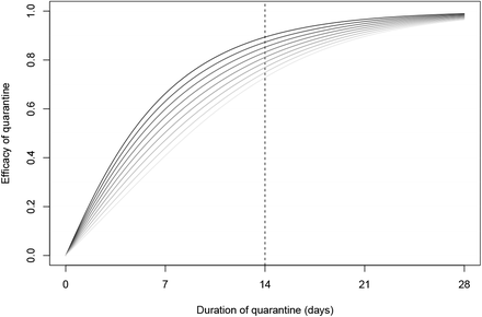
In order to investigate the effect of the duration tq of quarantine, as observed in Figure 6, we now quantify the efficacy of quarantine as the probability that a case that is initially unobservable becomes observable or recovers. Figure 7 shows the probability of success of quarantine (its efficacy c) as a function of its duration, for different values of the proportion π of asymptomatic and undetected cases. The curves here are obtained by using the method in B.6.
Probability c that the quarantine is successful as a function of its duration tq. From dark to light grey: fraction π of asymptomatic or undetected cases varying from 0.1 to 0.9 by steps of 0.1.
We observe that the probability c of success of the quarantine increases with the duration of quarantine, as could be expected. Furthermore, from Figure 7, testing helps the success of quarantine. Indeed, consider for instance the most widely used duration of quarantine: two weeks. If 90% of cases are asymptomatic or undetected, as could happen in a location making no effort to follow people during their isolation, the efficacy of quarantine would be about 70%. Efficacy would reach 90%, on the other hand, if only 10% of cases went undetected.
Note that the effect of quarantine on the rate of importation is derived directly from the efficacy c of quarantine. If λ is the rate of importation prior to quarantine and λq is the quarantine-regulated rate of importation, then λq = (1 − c)λ. Consider Figure 5, whose abscissa is expressed in units of 1/λ. The effect of a quarantine with efficacy c is to scale the days between importations right by a factor of 1/(1 − c). Consider a jurisdiction receiving a case on average every five days. A 50% efficacious quarantine leads to receiving one case every 10 days on average, while a 90% efficacious quarantine leads to receiving one case every 50 days on average.
4 Discussion
The main results of this study are summarised by Figure 5, where the proportion of successful importations is given as a function of the effective reproduction number  and the average number 1/λ of days between importations, and Figure 7, which shows the probability that quarantine is successful as a function of its duration tq. We use
  as a measure of the effort of local public health authorities.
For an initially susceptible population, the probability of an outbreak increases with the rate of importations, even when  , so that with importations every few days or less, outbreaks are almost certain, regardless of local efforts. However, the resulting attack rates increase with
  . With the parameters chosen for simulations, if case importations occur more than once every 10 days on average, then using measures to reduce
  to 0.5 still gives a 90% chance of outbreak, but with an attack rate of less than one percent at the end of three months. Thus, at the beginning of the spread, it is crucial to first hinder the importation of new cases in the location to reduce drastically the chance of an outbreak.
The sensitivity of the efficacy of the quarantine to its duration and to monitoring effort seen in Figure 7 and the resulting scaling of importation rates have important policy implications. A location receiving few cases because it is connected only to places with zero or low prevalence could reasonably adopt a shorter (seven to ten day) quarantine period and still achieve a large right scaling on the importation risk (Figure 5), provided it also implements a high level of follow up of quarantining individuals. Locations receiving cases at a high rate will need to ensure that quarantine is longer and with high compliance with the imposed duration, since noncompliance is equivalent to imposing shorter quarantines.
Our results apply to populations that see very few or no cases at all. They can however be applied to places seeing more cases if appropriate contact tracing allows to distinguish between cases stemming from imported cases and community generated cases. They can also be applied in general, but it will then be difficult or impossible to distinguish, as we do here, between cases generated by importations and community transmitted cases. Note that our results are also robust to the values used for parameters. We chose to use parameters mostly stemming from other work we have carried out on COVID-19, but we could also have used values from the now abundant literature on the subject. This would modify some of the graphs in a limited manner but would not alter our conclusions. We will make some of our code available on Github so it will be easy for readers to tailor our results to their specific situation. The approach used here allows to focus on the rate at which cases are imported and is in this sense quite different from other published work on the topic, which amalgamates several distinct components. It is useful, though, to provide some sense of the type of rates one can expect to observe. A formula and some examples are provided in Section A.5.
Data Availability
R code will be added to the Github repository.
Declarations of interest
None.
Funding sources
JA, SP and JW are supported in part by NSERC Discovery Grants. JA and JW are supported in part by CIHR. JA was supported in part by the Public Health Agency of Canada. JW is supported in part by the New Brunswick Health Research Fund. The sponsors played no role in the design of the study nor in the decision to submit this work.
Electronic supplementary material
A Methods
A.1 Mechanisms of spatialisation of epidemics and the nature of importations
We give here more details about the notions summarised in Figure 2 concerning the spatialisation of epidemics. Also, we make explicit the definitions regarding importations used in all the work.
Transportation is the actual movement of an infected individual to a new location. Importation occurs when an infected individual having acquired their infection in one location arrives in a different location while still infected with the disease. There can be two outcomes to an importation event; our terminology uses the point of view of SARS-CoV-2, the ætiological agent of COVID-19.
An unsuccessful importation is one that does not lead to any further local transmission. Note that unsuccessful importations usually are not detected. It is possible that a location will see many unsuccessful importation events before it actually detects one.
A successful importation is one that leads to at least one local transmission event, i.e., where the import case becomes the origin of one or more local transmission chains.
Amplification is then a critical phase of propagation that typically follows a successful importation. During amplification, cases multiply within a community, usually exponentially. In view of this, we define the severity of a successful importation as follows.
A noncritical successful importation results in local chains of transmission that are not sustained, i.e., a minor outbreak. Case counts remain low before eventually dying out. As for unsuccessful importations, some of these local chains of transmission might go completely unnoticed.
A critical successful importation sees sustained local chains of transmission. This is a major outbreak.
Finally, exportation is the process through which a community that is seeing some local transmission becomes the source of transportation events. Note that exportation does not require amplification to be taking place, although amplification does increase the probability that an individual leaving the community is harbouring the pathogen.
In our classification, exportation and transportation are very closely related. They are, however, considered as separate processes because they provide different entry points into the control of the spatial spread of COVID-19. Here, some methods of control of the spatial spread of an epidemic are listed.
Acting on transportation involves limiting the number of individuals hailing from known exporting locations that are allowed to enter one’s jurisdiction. In the case of COVID-19, this has taken the form of partial or complete travel bans.
To minimize the chance that, were an importation to occur, it be a successful one, most jurisdictions imposed a quarantine for travellers inbound from other locations. Some jurisdictions also implemented entry screening.
Once successful importations occur, jurisdictions used a variety of non-pharmaceutical interventions (NPI) to limit spread, i.e., curtail the amplification phase.
A.2 Structure of the epidemiological model
The structure of the epidemiological model is a slight modification of the SLIAR model in,1 itself a modified version of the SLIAR model in.2 The flow diagram is as shown in Figure ES.8: susceptible individuals, upon infection, move to the latent compartment. (Incubation and latent periods are assumed to overlap.) When their latent period is over, they can either progress to a symptomatic infection or to an asymptomatic one. At the end of the infectious period, individuals are removed; they no longer spread the disease.
Flow diagram of the SL1L2I1I2A1A2RI RAD model. Φ = β(I1 + I2 + ξ(A1 + A2)+ ηL2) is the force of infection. Blue compartments are observable, with I1 and I2 usually indistinguishable and observed as I1 + I2.
As in Arino & Portet,1 there are two each of the latent, symptomatically infectious and asymptomatically infectious compartments. This is so that the time of sojourn in these disease states is Erlang distributed; see B.3. Also, the force of infection Φ includes contributions not only from symptomatic infectious I and asymptomatically infectious A individuals but also from individuals in L2. This is to accommodate observations of pre-symptomatic COVID-19 infections.3 Finally, contrary to,1 the removed compartment is further subdivided into compartments for individuals having recovered from symptomatic and asymptomatic infections, RI and RA, respectively, and those having died from the disease, D.
Symptomatically infectious individuals are those who present symptoms and should normally be detected through testing, i.e., individuals who appear as confirmed cases in the data. Asymptomatically infectious individuals include those who are asymptomatic in the usual sense, but also symptomatic cases that avoid detection because of lack of testing. In the perspective of response to a crisis, using a case detection-based definition for symptomatic and asymptomatic cases allows to tailor model outputs to the situation in the location under consideration. This is further enhanced by using compartments RI and D directly connected to published data.
One drawback from using a case detection-based distinction between symptomatic and asymptomatic cases is that the parameters involved (π, δ and η) must be understood as incorporating not only disease characteristics but also some information about the location under consideration. For instance, locations performing a lot of testing will typically have a lower proportion of individuals following the asymptomatic route, i.e., a lower value of π, than those doing less testing.
Some notation is introduced to make discussions simpler. Individuals of type  are those infected with the disease, i.e.,
  . The prevalence of infection at time t is then
  . Individuals of type
  are unobservable infected, i.e.,
  . Observable infected are
  . The prevalence of unobservable and observable infections are obtained like that of infected cases, by summing the corresponding state variables. We can also define sets
  and
and  for, respectively, total unobserved and observed cases, by adding RA to
  and RI and D to
  ; these will not be used here.
We refer to1 for some basic properties of the corresponding ordinary differential equations (ODE) model and just mention here that the effective reproduction number of the ODE version is
 where S(0) is the initial susceptible population.1 This formula is applicable to the stochastic model and is therefore useful to set some parameter values. It is used for instance when considering the intensity of NPI measures in the local community.
A.3 Base model with a single importation event
Let t ∈ [0, ∞) be a continuous variable (time). The random vector V(t) defined as
 is the state of the system at time t. Denote ΔV(t)= V(t +Δt) − V(t) the change in system state in the time interval [t, t+Δt], with Δt> 0 sufficiently small to have at most one change during this interval. The probability of a transition is
 where ΔV(t) = (ΔS, ΔL1, ΔL2, ΔI1, ΔI2, ΔA1, ΔA2, ΔRI, ΔRA, ΔD). The components ΔS, ΔL1,…, ΔD take only the values ±1 and 0 because of the hypothesis on Δt being small enough. Transition probabilities are defined as follows (only nonzero values are shown):
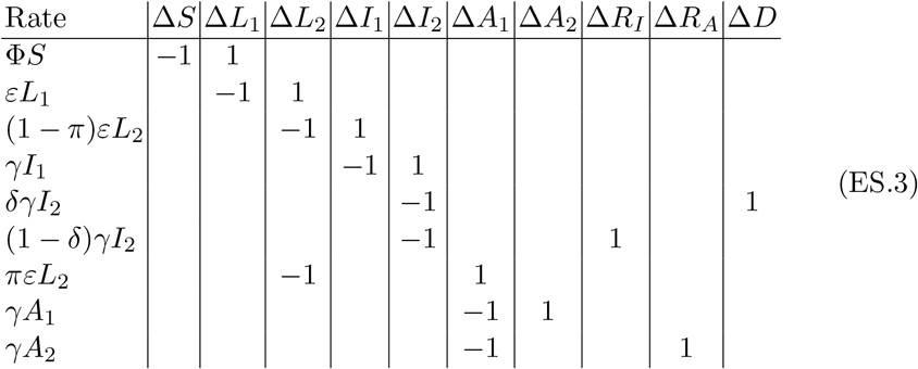
Parameters are β, the transmission coefficient, η and ξ the modifications of infectiousness for individuals who are, respectively, pre-symptomatically and asymptomatically infectious. A fraction π of individuals moves into an asymptomatic phase following incubation (and correspondingly, 1 − π develop symptoms or are detected). Because of the interpretation that we make of the symptomatic cases being those that are effectively detected, π is in essence a combination of the proportion of cases that are asymptomatic and those that are symptomatic yet avoid detection.
Finally, ε and γ describe the rates at which incubation and infectiousness end, respectively. The fraction δ is the case fatality ratio; it is assumed that asymptomatic cases are mild and never lead to death.
Model (ES.3), when it is used to consider single introduction events, is combined with initial conditions at time t = 0 of the form S(0) = S0 (the initial susceptible population), RI (0) = RA(0) = D(0) = 0 and one or several of L1(0),L2(0),I1(0),I2(0),A1(0) or A2(0) containing an integer number of individuals. In most cases, we consider the importation of a single individual, although in Section 3.1.2 we consider the effect of introductions of more than one infected individual.
When considering importations of a single infected individual at time t = 0, explicit formula can be derived concerning probabilities of events affecting individuals. For instance, suppose that importation is of a single infected individual in the L2 compartment, i.e., L2(0) = 1 with all other infected compartments empty. The probability that this individual recovers or dies from the disease without ever transmitting the virus is

The first term is the probability of progression from L2 to I1 without local transmission. The second one is the probability of progression from I1 to D or RI without local transmission. The third term is the probability of progression from L2 to A1 without local transmission and the last term is the progression from A1 to RA without local transmission.
A.4 Adding repeated importations to the model
A case importation event is described by three components: the time at which the event occurs, the size of the importation (the number of cases imported simultaneously), and the type (epidemiological status) of cases that are imported. In order to better understand the role of the rate of importation and lower the number of parameters affecting the output of the model, we suppose here that all importations are of size 1 and focus on the rate (timing) and nature (type) of importations.
The timing of importations is described using a Poisson process with a parameter λ; the mean time between importation events is 1/λ. An imported infected individual can belong to one of the six compartments L1, L2, I1, I2, A1 or A2; the infectious status of the imported individual is the type of the importation event. The probability of each type is given by  ,
,  ,
,  ,
,  ,
,  and
and  where
where  .
.
So the model with repeated importations is the CTMC with transition rates given by (ES.3), with initial condition S(0) = S0 and all other compartments zero, to which the following transitions are added.

A.5 Estimation of importation rates
The number per day of case arrivals in destination from origin i can be approximated by:

In general, a given location is connected to many other locations, say, N of them. Using (ES.6), we obtain a value λi for each of the i =1,…,N locations that are potential sources of importation for the location under consideration. As arrival times are Poisson distributed, from the perspective of the receiving location, arrival times of events are independent exponentially distributed random variables. As a consequence, the parameter of the Poisson distribution for a location is obtained by considering competing risks and

A.6 Characterising outbreak severity
To define the severity of the outcome, a threshold τ is chosen by adapting the results developed by Whittle19 for a simpler stochastic SIR model. Whittle establishes that the probability of a major outbreak for an SIR model is  if
if  , while no major outbreak is possible when
  , where I(0) is the initial number of infected individuals in the population. He also establishes the probability of a minor outbreak when
  , but this is not used here as we employ a different method for detecting minor outbreaks. Rather than computing the probability of a major outbreak, we decide on a probability p (in practice, p =0.95) of observing a major outbreak and set the threshold
  . This threshold is then interpreted as follows: suppose that during a simulation, we observe a successful importation; if at some point following the importation, the prevalence of the disease increases to or past τ, then with probability p,a major outbreak occurs.
As a consequence, we classify the type of importation events as follows.
A successful importation sees an S → L1 transition for a local susceptible individual.
An unsuccessful importation event does not lead to such a transition.
A critical successful importation is detected by checking, when
 , whether for some t ∈ [0,tf], the prevalence of infection
  . There is no major outbreak (and thus no critical successful importations) for
  .
.A noncritical successful importation is a successful importation that is not critical.
Severity can be further evaluated using observable infected cases  , unobservable infected cases
  , and total prevalence of infection
  .
.
B Results
The examples that follow use the data for Prince Edward Island (PEI). Although not completely homogeneous, PEI is small in surface area (5,660 square kilometres) and quite densely populated (25 inhabitants per square kilometre). PEI can be reached by plane, ferry and through a bridge linking it to the continent (the Confederation Bridge). PEI has, to this point, had very few cases of COVID-19, most of them being imported.
B.1 Role of the nature of the import case
Proportion of simulations with unsuccessful (UI), noncritical (NSI) and critical (CSI) successful importations, as a function of the type of initial case.
Since L1 individuals are not yet infectious to others, their effect on the proportion of simulations going to local extinction is not different from introducing an L2 individual. Importation of an asymptomatic case is more likely to be unsuccessful; this is even more noticeable late stage asymptomatic A2 cases. Indeed, in the simulations, asymptomatically infected individuals are less infectious and those in A2 spend, together with those in I2, the least amount of time in the population (parameter values used in simulations are given in Table 1). The effect of the length of time spent in the population is also visible for symptomatically infectious individuals, as evidenced by the difference between proportions of simulations with local disease extinction for I1 and I2 imports. Note that the proportion of simulations with unsuccessful importation (UI) can be computed theoretically from equations such as (ES.4). For instance, taking an initial case L2, the probability that the individual dies or recovers from the disease without transmitting the virus is 0.5288 (resp. 0.4176 and 0.2351) for  (resp. 1.2 and 2.5) from (ES.4); compare these values with the values of unsuccessful importations for L2 in Table ES.3. In further simulations, we assume that I individuals cannot travel.
B.2 Time to detection of local cases after importation
We continue with single stimulation simulations and present here results not discussed in the main text. We take the example of importation at time t = 0 of an L1 individual; results are qualitatively similar for importations of other types, with only the time distributions varying.
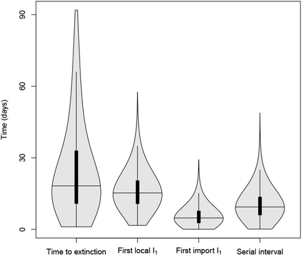
Time to extinction of the disease, first detected locally infected individual, first detected imported case, and serial interval. Base case simulation with S(0) = 142, 906 (population of Prince Edward Island), L1(0) = 1 and all other states equal to 0. Horizontal lines indicate the median value. Black rectangles are the inter-quartile range. Here,  .
.
In Figure ES.9, the first violin plot describes the distribution of local extinction times, the second shows the time distribution of the first local detected case, the third represents the time distribution of the first import detected case, i.e. when the import case L1 becomes I1. The distribution of serial intervals generated by the index case is shown on the right. Here, we define the serial interval as the length of time between the start of the simulation (i.e., the importation of an L1 individual) and the time at which the first local infection occurs (S → L1 transition).
The median time to the detection of the first symptomatic infection (I1 individual) following an importation event is 4.7 days (95% confidence interval 1.01 − 13.6) for the import case and 15.3 days (95% confidence interval 6.04−30.6) for a local case. In contrast, the first local infection event (S → L1 transition) occurs, on average, 9.4 days following an importation event (95% confidence interval 2.7 − 21.8), and more than 81% of these first infections occur after 5 days (roughly the median time of the first L2 → I1 transition).
Thus, if the import case is detected, this happens generally slightly before the first local transmission event takes place. In such a situation, the immediate isolation of the infected import case can prevent over half the local transmissions this individual would make. Note that this highlights the importance of quarantine: those transmissions that happen before isolation would not have taken place had this individual been quarantine. So quarantine is an efficacious way to compensate for delays in detection and isolation.
Most first detections of local I1 take place within 20 days following the importation of an L1 individual; however, in some situations, the first infected and detected I1 individual appears more than 30 days after the importation event. This characterises silent local transmission chains, i.e., ones involving only asymptomatically infected individuals.
B.3 Effect of the distribution of incubation periods
As mentioned in Section 2.1, compartments for L, I and A are subdivided in order to have Erlang distributed times of sojourn in these compartments rather than exponentially distributed ones. For instance, an individual traversing the two compartments L1 and L2 at the rate ε spends an average time 2/ε between entry into L1 and exit from L2, with their time of sojourn Erlang distributed.
Between the incubation and infectious periods, the average COVID-19 patient spends an average of 15 days infected. The time horizon for the present work and for other work on COVID-19, on the other hand, is short. With such commensurate time scales, the variance of distributions becomes important. Several papers have considered distributions of incubation periods.4, 5 Early work on 181 patients outside Hubei province before 24 February 20204 found the best fit for the distribution of incubation times for these patients to be an Erlang distribution with shape parameter (the number of compartments needed in our approach) equal to six. In order to judge the effect of using more compartments to obtain a better shaped distribution of incubation times, we ran the same simulations as in Table ES.3, with six L compartments instead of two as in the rest of this work. Results are shown in Table ES.4; the model is robust to the number of latent compartments used.
Proportions of simulations with unsuccessful (UI) and noncritical successful (NSI) importations, as a function of the type of initial case, when Rt =1.2. n is the number of latent compartments used in the simulations.
B.4 Estimation of importation rates
As some of our numerics is inspired by the example of Prince Edward Island (PEI), let us continue with this. The first day of the “Atlantic bubble”, where residents of all Maritime provinces of Canada were allowed to travel freely between these provinces, 8,500 people used the Confederation Bridge, which links PEI to the continent (in New Brunswick), going towards PEI. Suppose that cases in this flow happen with the same rate as in the general population and that prevalence in the general population can be deduced from confirmed case counts.
Assume that all travellers to PEI that day came from New Brunswick and that this relaxation of travel restrictions happened when New Brunswick experienced its highest number of active cases, on 2 April 2020, when there were 72 active cases.6 The estimate of the population of New Brunswick for the second quarter of 2020 was 780,890,7 i.e., a fraction of active cases of 0.000092202. Estimates for the prevalence of asymptomaticity vary; however, let us use the figure we have used throughout: 20%. Based on (ES.6), this gives 0.156744228 expected cases that day or, in other words, a mean time between importations of about 6.4 days, implying a rather high risk of importation (see Figure 5).
In practice, the Atlantic Bubble was put in place on 3 July 2020, at which time there was 1 active case in New Brunswick. Reasoning the same way, the mean time between importations in this instance would be of about 460 days, giving a very low risk of importation.
B.5 Effect of importation rates on outbreak severity
Using the threshold τ derived from Whittle,19 we investigate in Figure ES.10 the proportion of simulations with critical successful importations when  .
.
Proportion of critical successful importations (CSI) in a 3 month period for different values of the average number of days between two importations and  , an indicator of NPI efficacy.
B.6 Effect of post-arrival quarantine
The efficacy of quarantine can be expressed as the complement of the probability that an imported case is still in one of the unobservable infected states L1, L2, A1, or A2 at the end of the quarantine time tq, i.e., the probability they emerge from quarantine infected and undetected. Consider the matrix of transition rates constructed from the entries of the first column of (ES.3), represented here as the table of transition rates between stages of infection:
Let T be the matrix whose entries are given in this table, and let tij denote the ith row jth column entry of T. The diagonal entries of T are the rates of exit from each stage, and tij with i ≠ j is the rate of transition from stage j to stage i. If we let pi(t) denote the probability a given individual is in stage i at time t then p(t) satisfies the differential equations  , whose solutions are the matrix exponential eTt. Specifically, entries of eTt are the probabilities an individual is in the corresponding row-stage at time t conditional on having started in the corresponding column-stage at time 0. Figure 6 gives a graphical representation of eTt with parameters specified in Table 1 and t set to 7 days and 14 days respectively. Specifically, the entries of e7 T are as follows:
An individual in stage L2 at time 0 is distributed at time t = 7 according to column 2 of the table.
If an infected individual with state distributed according to pX arrives in a community at time 0 and is placed in quarantine for a time tq, then that individual’s state at time tq has distribution  . Further, the probability the individual is in one of the states in {L1,L2,A1,A2} at time t is given by
  where u is the characteristic vector for undetected infections, u = (1, 1, 0, 0, 1, 1, 0, 0, 0) and a range of times tq. If, after tq days, the individual is still in an unobservable state
  , then quarantine has failed. Otherwise, quarantine is considered a success. Recall that, in the model, I individuals have been detected by the authority, explaining why I1 and I2 individuals are considered as a success of the quarantine. We define the efficacy of quarantine, c, as the probability,
 that the imported case is in either an observable state, I1, I2, RI, or D, or recovered in state RA. Figure 7 represents c for different values of tq, where ueTtqpX is computed for pX = (0.25, 0.25, 0, 0, 0.25, 0.25, 0, 0, 0)T.
Furthermore, the quarantine-regulated importation rate λq is expressed by


