FOCUS: Forecasting COVID-19 in the United States

2.1 Data Sources

The first step for the FOCUS effort was to identify a reliable data source for incident and cumulative counts of cases and deaths in the United States. For our forecasts, we relied on daily count data curated in the COVID-19 Data Repository by the Center for Systems Science and Engineering (CSSE) at Johns Hopkins University (Dong, Du, and Gardner 2020). In initial efforts, we also explored the New York Times³ COVID-19 repository, however we chose to solely use the JHU CSSE data given that the COVID-19 Forecast Hub organizers consider it the source of truth data for model evaluations.

During the FOCUS project period, the JHU CSSE group maintained daily count data posted as .csv files in a GitHub repository.⁴ Data were collated from public health agencies across the United States, and were made available at the county level. We developed code to programmatically read the .csv files with confirmed cases and deaths directly from GitHub, and then aggregate daily data to weekly counts. The code is written to parameterize granularity at which the counts are aggregated. For example, a state-level aggregation would add up all daily cumulative counts from counties to arrive at a daily cumulative count for the state. From there, the cumulative count is translated to an incident count by subtracting the cumulative count of the prior day from that of the current day. Daily incident counts are summed to weekly incidence, from which weekly cumulative counts are then calculated. Note that each week is translated to “epiweek” (MMWR week)⁵ format prior to modeling.

2.2 Statistical models

We employed a time series approach (SigSci-TS) to forecast incident cases, incident deaths, and cumulative deaths. For case data, we first retrieved the JHU CSSE weekly incident case counts using the methods previously described. We then fit a non-seasonal autoregressive integrated moving average (ARIMA) model using the historical case data. Parameters for p, d, and q (i.e. the orders for autogreressive terms, differencing, and moving average respectively) were selected using an automated parameter tuning process implemented in the fable R package (O’Hara-Wild, Hyndman, and Wang 2020a). After automatically performing a grid search of possible values for each order using the Hyndman-Khandakar algorithm (Hyndman and Khandakar 2008), the ARIMA model will use the combination of parameters that minimizes the corrected Akaike information criteria (AICc) (Cavanaugh 1997). Given that the process is automated and driven by the weekly dynamics of the input data, the specific parameters chosen for the incident case ARIMA model may differ weekly and/or by location. It is also worth noting that the fable R package allows for the parameter space to be arbitrarily constrained. Our initial models of national targets only used an unconstrained parameter space. After we included state-level targets we observed implausible forecast results for some states and subsequently restricted the space as follows: p = 1 or 2 ; d = 0, 1, or 2; q = 0. The parameters for P, D, and Q (seasonal orders) were all set to 0 to achieve an ARIMA fit without seasonality. After fitting the ARIMA model(s) each week (one for each location being included in the submission), we generated weekly forecasts of incident cases out to a four week horizon.

For incident death forecasts we used a time series linear modeling framework (TSLM). While the TSLM model can account for time series components (e.g. trend or seasonality), we did not specify any exogenous regressors. The fit for incident deaths used a three-week lag of incident case counts as the only predictor. Forecasts out to the four week horizon were generated by passing incident case counts at each horizon. Given that the lag does span the fourth week, we had to sequence forecasting to first generate one week-ahead incident case forecasts in order to create incident death forecasts for all targets. Forecasts of cumulative deaths were generated by summing the cumulative number of incident deaths reported the prior week with each of the incident death forecasts through the four week horizon.

All forecasts yielded point estimates as well as predicted values that divide the distribution at the following quantiles: 0.01, 0.025, 0.05, 0.1, 0.15, 0.2, 0.25, 0.3, 0.35, 0.4, 0.45, 0.5, 0.55, 0.6, 0.65, 0.7, 0.75, 0.8, 0.85, 0.9, 0.95, 0.975, and 0.99. Quantile estimates were generated by first converting quantiles to the bounds of the associated prediction interval, then creating intervals of each desired width before finally joining the predicted limits back to the appropriate quantiles. The quantiles above were chosen to meet the COVID-19 Forecast Hub submission requirements.⁶ To ensure non-negative estimates, predicted values were truncated at 0.

We fit incident case and incident death models using the ARIMA() and TSLM() functions from the fable R package (O’Hara-Wild, Hyndman, and Wang 2020a). Forecasts from fitted models were generated using the forecast() function in the fabletools R package (O’Hara-Wild, Hyndman, and Wang 2020b). We arrived at prediction intervals by using the hilo() function originally released in the distributional R package (O’Hara-Wild and Hayes 2020) and re-exported in fabletools.

2.3 Automation

All code to retrieve, pre-process, analyze, and format submission data was written in R (R Core Team 2019) and packaged in focustools.⁷ The package provides documentation for all functions and is built to include internal data, such as the names, abbreviations, and FIPS codes for the state, territory, and county locations in the United States. Using the focustools functions in R, team members were able to interactively generate forecasts and prepare the submission format using the quantile format described previously.

All of the forecasting code for the project was maintained under version control. Prior to interactively generating forecasts, team members could make sure they had up-to-date versions of the code. However, the interactive forecast workflow could become redundant or problematic if multiple team members were to independently create the weekly forecast submission files. It is possible that despite a common interface, individual users might pass arguments, enforce assumptions, or otherwise script the workflow such that they would arrive at different forecast results. To guard against this, we sought to automate as much of the forecasting workflow as possible.

The FOCUS automation relied heavily on cloud computing via Amazon Web Services (AWS). We leveraged several AWS features, including:

• Elastic Compute Cloud (EC2)⁸ to provision a templated computing instance that can run the forecast pipeline, as well as a separate instance to host a forecast exploration app.

• Launch templates⁹ to codify the provisioning of the pipeline and app instances.

• Elastic IP¹⁰ service to allocate and associate a static IP to the app instance.

• Simple Storage Service (S3)¹¹ for storing outputs from the forecast pipeline as well as software/scripts needed to provision the EC2 instance.

• Identity Access Management (IAM)¹² roles to provide access between services (i.e. Lambda to EC2 and EC2 to S3).

• Lambda¹³ to deliver a serverless function to launch the EC2 forecast pipeline.

• CloudWatch¹⁴ to manage the execution of the Lambda function on a weekly schedule.

2.4 Evaluation

Methodology for evaluating COVID-19 forecasts is rapidly evolving. With a range of targets, horizons, and locations, there are numerous endpoints to evaluate. Furthermore, the type of forecasting error may have differential meaning depending on the context. For example, either over or under prediction may be more costly in terms of public health impact, and the effect of one or the other may need to be taken into account during evaluation. In some cases a point estimate may be more beneficial given ease of interpretation. Lastly, a simple yes/no describing whether or not the observed value fell within a predicted range may be of interest.

We evaluated the performance of our forecasts using three complementary metrics that collectively address each of the scenarios above:

• Weighted Interval Score (WIS): Proper scoring rule for predictive distributions that weights quantiles and penalizes overprediction and underprediction.

• Mean Absolute Error (MAE): Absolute difference between predicted point estimates and observed values.

• Interval coverage: Binary as to whether or not the observed count fell within the forecasted interval.

The WIS was developed by some of the coordinators of the COVID-19 Forecast Hub as a mechanism to evaluate submissions. Details of the methods to calculate the WIS have been described previously (Bracher et al. 2021) and contextualized with other evaluation mechanisms such as MAE and interval coverage (Cramer et al. 2021). All of these metrics depend on a reliable data source for observed counts. The most widely used source of truth for COVID-19 outcomes in the United States is the repository curated by the JHU CSSE group (Dong, Du, and Gardner 2020).

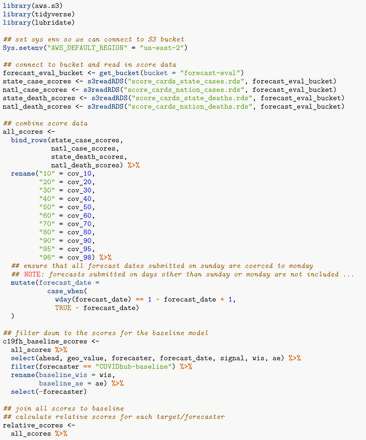
The WIS, MAE, and interval coverage metrics are all calculated for COVID-19 Forecast Hub submissions by the Carnegie Mellon University Delphi group.¹⁵ The scores are made available in a publicly-accessible AWS S3 bucket. We retrieved the pre-computed Delphi scores to evaluate the performance of our submitted forecasts. Scores were retrieved on 2021-05-10 and limited to submissions between January 11, 2021 and April 12, 2021. Each combination of forecast date, target, horizon, and location was assigned the following: WIS, MAE, and binary indicators as to whether or not the 50% and 95% prediction intervals covered the observed count. We summarized each metric by target, averaging across locations, forecast dates, and/or horizons. To rank the performance with respect to other participants, we computed a relative metric for WIS, MAE, and interval coverage by dividing our scores (and those of other participants) by the scores for the COVIDhub baseline model, which forecasts median incidence equal to the previous week (Cramer et al. 2021). For overall rankings (averaged across all locations, horizons, and forecast dates), we only included models that had at least 500 forecasts. The overwhelming majority of forecasts were submitted on Sundays or Mondays. All Sunday forecast dates were coerced to Monday in order to join with baseline model. A very small number of forecasts were not submitted on Sunday or Monday; the scores from these were not included in rankings. Code to retrieve and aggregate scores for rankings is available in the Appendix (A1).

3.1 Forecasts submitted

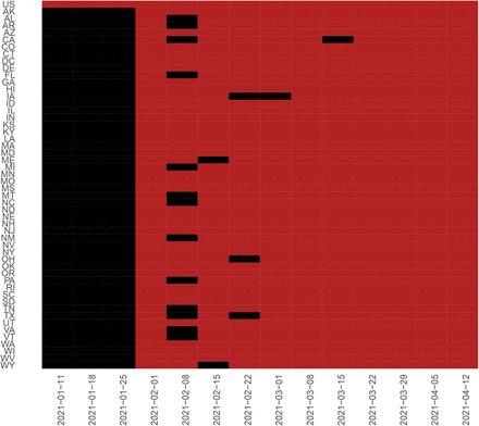
Between January 11, 2021 and April 12, 2021 we issued 14 submissions to the COVID-19 Forecast Hub, totaling 6,660 forecasts across three targets (incident cases, incident deaths, and cumulative deaths), four horizons (1 to 4 weeks ahead), and 52 locations (national, 50 states, and Washington DC). Figure 1 shows the locations for which forecasts were submitted each week. While initial forecasts were only made on the national level, the majority of weekly submissions included forecasts for state-level targets as well. For some weeks, we excluded certain states prior to submission due to implausible estimates. The cause of these inconsistencies was typically a backlog in reporting of cases in the given state, and we did not feel that it was appropriate to submit a forecast based on unreliable data for that week. Every forecast submitted included estimates of values at required quantiles and point prediction. All submissions were accepted by the COVID-19 Forecast Hub and included in the weekly ensemble models reported by the CDC.

• Download figure
• Open in new tab

Figure 1:

Weekly submission by location. Cells marked in red had 1-4 week horizons for incident case, incident death, and cumulative death targets included in the submission for the given week. Cells marked in black denote locations that were excluded from the weekly submission.

3.2 Automation

All functions to run statistical models, generate forecast outputs, prepare formatted submission files, and create tabular/visual summaries of forecasts are included in the focutools R package. The package is available on GitHub under the GPL-3 license and includes robust function documentation and narrative vignettes describing basic usage.¹⁶ By the end of the project, the package was used as part of the automated cloud pipeline. Figure 2 depicts the automation pipeline as implemented.

• Download figure
• Open in new tab

Figure 2:

Illustration of automation pipeline. The weekly workflow starts with a scheduled AWS CloudWatch event to trigger an AWS Lambda operation. The function can access IAM credentials to launch the pipeline instance from a template that includes bootstrapping code, storage specifications, and details for the instance to be run. When the forecasting instance starts, it installs necessary software, generates forecast output, writes submission-ready files to an S3 bucket, and then self-terminates. Another EC2 instance hosts a web app with access to the same S3 bucket, allowing users to interactively review and download forecast output prior to submission. After reviewing through the web app, users manually inspect and then download the validated submission file, commit the file to the fork of the COVID-19 Forecast Hub repo, and submit a pull request upstream, which triggers an automated validation process.

The weekly forecasting workflow began with a CloudWatch event (defined by a cron rule) to trigger a Lambda function. The Lambda function used a Python script calling the boto3¹⁷ AWS client with the instruction to launch the pipeline instance from a template. The launch template included specific instructions needed to provision the instance: availability zone (us-east-1), instance type (T2.medium), AMI (Ubuntu 18.04 OS), IAM role with read/write access to the project S3 bucket, behavior on shutdown (terminate), and a definition of additional storage to be attached (16GB). The template also included a Base64 string that encoded a Bash bootstrapping script. Details of the steps performed in the bootstrap are available in the Appendix (A2).

The design for the weekly forecasting pipeline prioritized ephemerality. The bootstrap commands were run once, and by the end of the script the EC2 instance that ran the workflow was terminated. At the same time the following week, a new instance was launched with an identical configuration and set of instructions. Each weekly run used the same S3 bucket, from which team members could retrieve error logs if there were pipeline failures.

Once the forecasts were generated, the contents were reviewed by the team for plausibility of estimates. Team members reviewed plots of forecast output and tabular summaries of the predictions. To streamline this review process, the automation stack included a second instance to host a web interface for visually inspecting, filtering, and downloading forecast submission files. The web interface was written in R as a Shiny application and delivered via a wrapper function in the focustools R package. As with the forecast pipeline, details of the instance hosting the app were defined in a launch template: availability zone (us-east-1), instance type (T2.small), AMI (Ubuntu 18.04 OS), IAM role with read/write access to the project S3 bucket, and a definition of additional storage to be attached (16GB). Details of the bootstrapping steps performed on instance launch are available in the Appendix (A3).

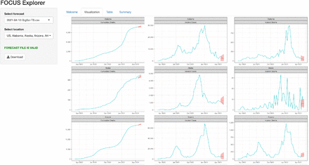
Note that unlike the pipeline instance, the bootstrap commands for the app host do not end with a terminated instance. In fact, the instance hosting the app was assigned a static IP allocated via the Elastic IP service and stayed running such that team members could access the interface at their convenience. The machine was configured to run a cron job every hour to refresh the contents of a directory synced from S3 containing all pipeline-generated forecast files. The app listed the contents of that directory and presented each file name as a selection in a drop-down. After selecting a forecast file from the drop-down, the user could view plots of the forecasted curve and review tables of predicted counts and percent change over the four week horizon. Each result was faceted to locations selected by the user (defaulting to all locations present in forecast file). When ready to submit, the user could export the validated .csv submission file directly from the web interface. Figure 3 is a screenshot of the FOCUS explorer app interface.

• Download figure
• Open in new tab

Figure 3:

Screenshot of FOCUS Explorer app. The FOCUS Explorer Shiny application ships with the focustools R package and can be run locally or can be hosted. When starting the Shiny application, users must provide historic time series data prepared with the data retrieval functions from the focustools package. The app allows users to interactively explore forecast output through visualizations of observed counts and forecasts and tabular summaries. Each plot is stratified by location and target. The user can restrict locations and download the data in validated COVID-19 Forecast Hub submission format.

3.3 Scoring

Table 1 details how SigSci-TS forecasts submitted between 2021-01-11 and 2021-04-12 ranked relative to other submissions to the COVID-19 Forecast Hub. Metrics were averaged across all locations (US and states/territories) and horizons (1-4 weeks). Models were only ranked if they had scores available for at least 500 forecasts (combined across locations, horizons, and forecast dates). In terms of WIS, our forecasts ranked 6 of 30 for incident cases and 16 of 41 for incident death targets. When evaluating with MAE on average the forecasts ranked 3 of 33 for incident cases and 39 of 45 for incident death targets. For coverage, 95.2% and 75% incident case forecasts included the observed count in the 95% and 50% prediction intervals respectively. 93.1% and 48.5% incident death forecasts included the observed count in the 95% and 50% prediction intervals respectively. Our incident case model ranked 3 of 29 in the 95% coverage and 1 of 29 in the 50% coverage. The incident death forecasts ranked 3 of 42 in the 95% coverage and 9 of 42 in the 50% coverage.

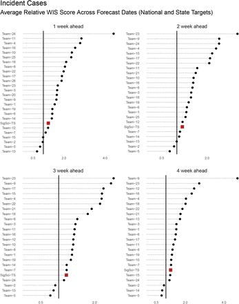
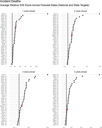
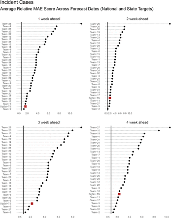
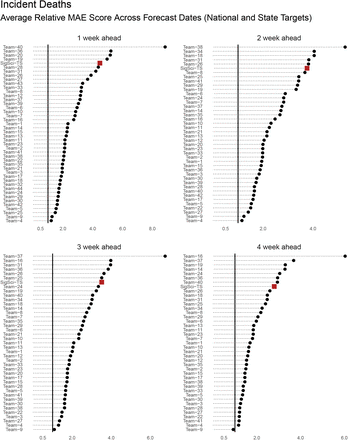
The rankings above were computed by averaging across all horizons. Figures 4-7 illustrate SigSci-TS performance in incident death and incident case forecasts for WIS and MAE metrics stratified by horizon (1-4 weeks).

• Download figure
• Open in new tab

Figure 4:

WIS rankings for incident case forecasts stratified by horizon. Scores are averaged across all locations and forecast dates (between 2021-01-11 and 2021-04-12) and calculated relative to the COVIDhub-baseline model. For this plot teams with less than 125 forecasts were excluded. One team was excluded from the plot because of extreme outlying scores. SigSci-TS is represented as a red square. The horizontal black line represents marks the relative score of 1 (i.e. the baseline model performance).

• Download figure
• Open in new tab

Figure 5:

WIS rankings for incident death forecasts stratified by horizon. Scores are averaged across all locations and forecast dates (between 2021-01-11 and 2021-04-12) and calculated relative to the COVIDhub-baseline model. For this plot teams with less than 125 forecasts were excluded. One team was excluded from the plot because of extreme outlying scores. SigSci-TS is represented as a red square. The horizontal black line represents a relative score of 1 (i.e. the baseline model performance).

• Download figure
• Open in new tab

Figure 6:

MAE rankings for incident case forecasts stratified by horizon. Scores are averaged across all locations and forecast dates (between 2021-01-11 and 2021-04-12) and calculated relative to the COVIDhub-baseline model. For this plot teams with less than 125 forecasts were excluded. Two teams were excluded from the plot because of extreme outlying scores. SigSci-TS is represented as a red square. The horizontal black line represents a relative score of 1 (i.e. the baseline model performance).

• Download figure
• Open in new tab

Figure 7:

MAE rankings for incident death forecasts stratified by horizon. Scores are averaged across all locations and forecast dates (between 2021-01-11 and 2021-04-12) and calculated relative to the COVIDhub-baseline model. For this plot teams with less than 125 forecasts were excluded. Two teams were excluded from the plot because of extreme outlying scores. SigSci-TS is represented as a red square. The horizontal black line represents a relative score of 1 (i.e. the baseline model performance).