Abstract
The effective reproductive number Re is a key indicator of the growth of an epidemic. Since the SARS-CoV-2 pandemic started, many methods and online dashboards have sprung up to monitor this number. However, these methods are not always thoroughly tested or are applied only to a limited geographic range. Here, we present a method for near real time monitoring of Re, applied to epidemic data from 170 countries. We thoroughly validate the method on simulated data, and present an intuitive web interface for interactive data exploration. We show that in the majority of countries the estimated Re dropped below 1 only after the introduction of major non-pharmaceutical interventions. For Europe, Asia, and North America we found that the implementation of non-pharmaceutical interventions was associated with reductions in the effective reproductive number. Globally, we found that relaxing non-pharmaceutical interventions did not fully revert Re values to their original levels. Generally, our framework is useful both to inform governments and the general public on the status of the epidemic in their country, as well as a source for detailed comparison between countries and in relation to local public health policies and external covariates such as mobility, behavioural, or weather data.
Significance statement During the SARS-CoV-2 pandemic, governments need a way to monitor the epidemiological situation in their country. A key indicator is the effective reproductive number Re. It describes the average number of secondary infections caused by a primary infected individual. Here, we present a method to estimate Re from case report data. We thoroughly validate the method on simulated data, and present Re estimates for 170 countries on an interactive web interface. We then use this method to investigate the impact of non-pharmaceutical interventions on reducing Re worldwide. We find that the estimated Re was significantly above 1 prior to the introduction of major non-pharmaceutical interventions, and that relaxing these interventions does not fully revert Re estimates to their prior levels.
1 Introduction
During an infectious-disease outbreak, such as the ongoing SARS-CoV-2 pandemic, accurate monitoring of the epidemic situation is critical to the decision-making process of governments and public health authorities. The magnitude of an epidemic, as well as its spatial and temporal infection dynamics determine the exposure risk posed to citizens in the near and long-term future, the pressure on critical infrastructure like hospitals, and the overall burden of disease to society.
The effective reproductive number Re is a key indicator variable to describe how a pathogen spreads in a particular population [1, 2, 3]. It quantifies the average number of secondary infections caused by a primary infected individual. It also has a natural threshold value of 1, below which the epidemic reduces in size [1, 4]. Re typically changes during the course of an epidemic as a result of the depletion of susceptible individuals, changed contact behaviour, seasonality of the pathogen, or the effect of pharmaceutical and non-pharmaceutical interventions (NPIs) [1, 5, 6, 7, 8].
Different methods have been developed to estimate the effective reproductive number. They broadly fall into two categories: those based on compartmental models, e.g. [5, 9, 10], and those that count the number of secondary infections per infected individual directly, based on a time series of infection incidence, e.g. [11, 12]. We focus on the latter methods, in particular the EpiEstim method of Cori et al. [12], as they rely on only few, simple assumptions, are less prone to model misspecifications, and well-suited for near real-time monitoring of the epidemic [13].
The infection incidence based methods face the difficulty that infection events cannot be observed directly [13]. These events can only be surmised with a certain time lag, e.g. when individuals show symptoms and are tested, via contact tracing, or via periodic testing of a cohort of individuals [4]. To use these methods, one must thus employ a proxy for infection events (e.g. the observed incidence of confirmed cases, hospitalisations, deaths). This proxy is either used directly in lieu of the infection incidence, or it is used as an indirect observation to infer past infections [13]. A benefit of the infection incidence based methods is that they can be applied to multiple proxies of infection events independently, allowing for direct comparison of the inferred results for the same epidemic [6]. However, depending on the method used to infer infections from the observed incidence time series, one can also introduce biases such as smoothing sudden changes in Re [13, 14, 15].
Several methods, software packages, and online dashboards have been developed to monitor Re during the SARS-CoV-2 pandemic (e.g. [16, 17, 18]). A pipeline for the continuous monitoring of Re using infection incidence based methods should include four critical steps: (i) gathering and curation of observable proxy data of infection incidence, (ii) reconstruction of the unobserved infection events, (iii) Re estimation, and (iv) communication of the results, including uncertainty and potential biases. These are four axes that also define the differences between existing methods. During the SARS-CoV-2 epidemic, many local public health authorities have made case data publicly available. Depending on the data sources used, Re reports span different geographical scopes, from the scale of a city, region, country, or the entire globe [17, 19, 20]. The second step, i.e. going from a noisy time series of indirect observations to an infection incidence time series, is technically the most challenging. Biases can be introduced easily, and accurately assessing the uncertainty around the inferred infection incidence is a challenge in itself [13]. For the third step, i.e. to estimate Re from a timeline of infection events, there are ready-to-use software packages [12, 21], which produce unbiased Re estimates along with an estimate of the uncertainty resulting from this step. Finally, the communication of results to the general public and decision makers is essential, but is often overlooked.
We present a pipeline, together with an online dashboard, for near real-time monitoring of Re. We use publicly available data gathered by different public health authorities. Wherever possible, we show results obtained from different types of case reports (confirmed cases, hospitalisations or death). This allows comparison across observation types and hence a better assessment of the validity of the estimates. Results are updated daily, and can be found on https://ibz-shiny.ethz.ch/covid-19-re/.
Because Re estimates reflect changes in virus transmission dynamics, they can be used to assess the impact of public health interventions. Prior work on the relative impact of specific non-pharmaceutical interventions on Re has shown conflicting results [8, 22, 23, 24, 25, 26]. These differences can be attributed mostly to different model formulations [24, 27], including differing assumptions on the independence of NPIs [27], differing timescales over which the effect of the NPI was analysed [8, 25], whether the time point of the NPI was assumed fixed or allowed to vary [26], and differing geographical scope.
There is a need to address whether the strength of measures and the speed of their implementation resulted in a larger and faster decrease in the Re, and specifically whether highly restrictive lockdowns were necessary to reduce Re < 1. Further, it remains unclear how the impact of interventions differed across time and geographical regions. We add to this debate by using our global Re estimates across timescales that include the lifting of many NPIs. While we cannot determine causal relationships, we use our method to assess likely associations.
2 Results
A new pipeline to estimate the effective reproductive number of SARS-CoV-2
We have developed a pipeline to estimate the time-varying effective reproductive number of SARS-CoV-2 from observed COVID-19 incidence time series (see Materials and Methods). We build upon the existing EpiEstim method [12] to estimate Re(t) from a time series of infection incidence. To infer the infection incidence from a time series of (noisy) observations, we extended the deconvolution method by Goldstein et al. to deal with partially observed data and time-varying delay distributions [13, 14]. To reduce numerical artefacts resulting from the noisy nature of these observations, we smooth the data prior to deconvolution. We take into account uncertainty in the observation process using a bootstrap procedure, and in the Re estimation using the 95% highest posterior density intervals from EpiEstim. As observed incidence data we use COVID-19 confirmed case data, hospital admissions, and deaths (with type specific delay distributions, see Materials and Methods).
Validation on simulated data
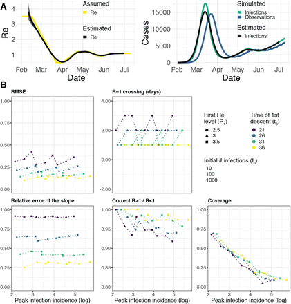
The method was validated with simulations of several epidemic scenarios (Materials and Methods section 4.5). For each scenario, we specified an Re time-series, from which we simulated infection and observation incidence. Then, we used our method to infer the infection incidence and Re from the observation incidence, and compared to the true underlying Re values (Fig. 1A). The specified Re trajectories were parametrised in a piecewise linear fashion, where we fixed the plateau values for Re and the time-points at which the trajectory changed slope. To mimic the course of the epidemic observed in many European countries in spring and summer 2020 [28], we started with Re values around 3, then dropped to a value below 1 (the ‘initial decrease’), to subsequently rise slightly above 1 for some time (Fig. 1).
The left panel shows the specified Re trajectory (yellow line) with five plateaus Re = (3.5, 0.5, 1.2, 0.95, 1.1) and the estimated Re trajectory. The right panel shows the simulated infections (in green; initial infection incidence I0 = 10), and the case observations (in blue) simulated from those infections. The infection incidence inferred from the case observations is shown in black. The trajectory shape mimics the course of the epidemic observed in many European countries, which started with an Re ∼ 3, then dropped to a low value below 1 (the ‘initial decrease’), to subsequently oscillate around 1 for some time. (B) Performance of our method on simulated scenarios. From top to bottom, left to right, we show: (i) the normalised root mean squared error (RMSE), (ii) the error of the slope of the first decrease, (iii) the delay of the mean crossing Re = 1, (iv) the fraction of time points for which we correctly infer that Re is significantly above or below one, (v) the coverage of the true Re value. These metrics are further described in Materials and Methods section 4.5. In the scenarios we varied the initial Re level (R1; point shape), the time of the first descent (t3; point colour), and the number of initial infections (I0∈ {10, 100, 1000}; not indicated separately as it determines the peak infection incidence directly). In these simulations a shorter Re time series was used than in panel (A), with three plateaus: R2 = 0.5, R3 = 1.2.
The results show that our method allows accurate monitoring of the effective reproductive number across the entire length of the time series (Fig. 1B; metrics described in Materials and Methods section 4.5). The low root mean square error (RMSE) indicates that our estimates closely track the true Re value. In the simulated trajectories, the slope of the initial decrease can be correctly inferred, although the relative error is greater for steeper slopes (Slope error). More importantly, we correctly infer whether Re is significantly above or below 1 for 95% of the time series (Correct R > 1/R < 1), and across all simulations we miss the date of the R = 1 crossing by at most 3 days (R = 1 difference; calculated between the Re point estimate and the true Re).
The minor misestimation of the slope is primarily due to the smoothing step included in our deconvolution algorithm. However, the inclusion of smoothing greatly improves our performance across more realistic scenarios with daily or weekly observation noise (Supplemental Fig. S1). With smoothing, the performance of our method is mostly independent of the amount of observation noise (Supplemental Fig. S2). When the mean of the delay distribution between infection and case observation is misspecified, we can still determine the shape of the Re curve, but do misestimate when Re = 1 (Supplemental Fig. S3). Further model misspecifications, such as a wrong generation time interval, have been investigated by Gostic et al. [13].
The fraction of the Re time-series where the true value of Re falls within our estimated confidence intervals (the ‘coverage’), decreases strongly for larger overall infection incidence. This indicates that the confidence intervals are too narrow for large case numbers. This result is consistent across all scenarios, independent of the slope of the initial decrease (Fig. 1B) or the delay distribution used (data not shown). We are improving the bootstrapping method further to account for this variance.
Our method clearly outperforms the common approach of using a fixed delay to infer the infection incidence time series (Supplemental Fig. S5). Our ability to allow for empirical, time-varying distributions in the estimation also slightly improves the estimated Re (Supplemental Figs. S4a, S4b), especially when strong time variation is present.
Monitoring Re during the COVID-19 pandemic
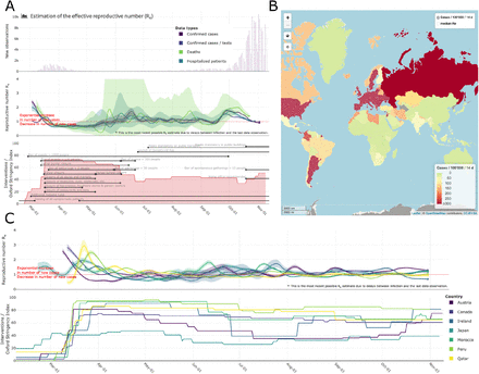
We apply this Re estimation method to COVID-19 case data from 170 countries (Fig. 2). All estimates are updated daily and made publicly available on an online dashboard https://ibz-shiny.ethz.ch/covid-19-re/ (results available for download). For most countries, we include multiple observation sources, such as daily incidence of COVID-19 cases and deaths, and, when available, hospitalisation incidence.
(A) Swiss cases, Re estimates, timeline of non-pharmaceutical interventions (NPIs), and stringency index. (B) World map of incidence per 100’000 inhabitants over the last 14 days. (C) Comparison of Re estimates across a handful of countries, with timelines of stringency indices. All panels were extracted on Nov. 13 2020. Dashboard url: https://ibz-shiny.ethz.ch/covid-19-re.
The online app allows for comparison through time within a single country, between multiple observation traces, or between multiple countries. The data download further allows users to put these estimates in relation to external covariates such as mobility, weather, or behavioural data. The map view enables comparison across larger geographical areas and additionally reports the cases per 100’000 inhabitants per 14 days.
Fine-scale data allows fine-scale analysis: the example of Switzerland
When detailed epidemiological data about individual cases (i.e. line lists) is available, we can increase the precision of our method by relaxing two assumptions: (i) distributions of delays between infection and observation do not change through time and (ii) outbreaks occur in a well-mixed homogeneous population at the country-level. In particular, we collaborated with the Federal Office of Public Health (FOPH) in Switzerland to further refine the monitoring of the Swiss SARS-CoV-2 epidemic.
The FOPH line list data contains information on the delays between onset of symptoms and reporting (of a positive test, hospitalisation or death) for a significant fraction of the reported cases. We estimate the time-varying empirical delay distribution from this data and use it as input to the deconvolution step, instead of estimates of these delays from the literature (for details see Materials and Methods section 4.2). The delay distribution is thus tailored to the specifics of the Swiss population and health system. Moreover, each distribution varies through time and thus reflects changes caused by e.g. improved contact tracing or overburdened health offices (see Fig S6; Supplementary Discussion). Whenever available in the FOPH line list, we use the symptom onset date of patients as the date of observation and thus only deconvolve the incubation period to obtain a time series of infection dates. The effect of these modifications is relatively minor in most parts of the estimated Re curve (see Fig. S7), yet the difference between Re point estimates for a particular day can be as big as 20%.
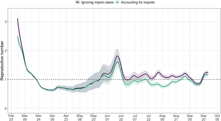
Using FOPH data on the fraction of cases infected abroad, we can correct our Re estimate for imports to reflect only local transmission. This is especially important in phases during which the local epidemic is seeded from abroad, and local transmission occurs at a low rate relative to case importation (Fig. S8). Since we do not have data on the number of cases infected in Switzerland and then “exported” to other countries, we cannot correct for exports. Thus, the estimated Re value corrected for imports is a lower bound for the Re estimate which would be obtained if we could account for the location of infection of all cases detected in Switzerland or exported out of the country.
In the majority of countries the critical threshold R=1 was crossed only after the implementation of nationwide lockdowns
With our method, we can now assess the association between non-pharmaceutical interventions (NPIs) and the effective reproductive number Re. We selected 20 European countries for which the reported data was free of major gaps or spikes (as these are indicative of low-quality reporting), and for which we could estimate Re prior to the nationwide implementation of a lockdown. The dates of interventions were extracted from news reports (sources listed in Supplementary Table S2), and ‘lockdown’ taken to refer to stay-at-home orders of differing intensity. Of the countries investigated, all except Sweden implemented a lockdown (19/20). We estimated that Re was significantly above one prior to the lockdown measures in nearly all countries with a lockdown (17/19; Table 1). Only Denmark, which had a complex outbreak consisting of two initial waves, had an estimated Re significantly below one prior to this date. We showed on simulated data that our method estimates the date of the Re = 1 threshold crossing with up to 3 days delay. Accounting for these 3 days does not change our results (Table 1). The results are also remarkably consistent across the different observation types (Supplementary Table S1). However, the confidence intervals tend to be wider for the estimations based on the death incidence because the number of deaths is much smaller than the number of cases, and the relative noise in observations tends to be higher.
Based on news reports, we report when a country implemented stay-at-home orders (a ‘lockdown’). We determined when the Re estimate and its confidence intervals first dropped below 1. Of the investigated countries that implemented a nationwide lockdown, only two (Denmark, Slovenia) had Re estimates that included or were below one before a nationwide lockdown was implemented. ‘Time until R < 1’ indicates the number of days between the lockdown and the date that the mean Re < 1.
To consider this question for countries outside of Europe, we used the stringency index (SI) of the Blavatnik School of Government [29] to describe the public health response in different countries (Fig. 3a). This is a compound measure describing e.g. whether a state has closed borders, schools, or workplaces. For example, a country with widespread information campaigns, partially closed borders, closed schools, and a ban on public events and gatherings with more than 10 people would have an SI slightly above 50. As reference date, we determined when a country first exceeded a stringency index of 50 (tSI50). Then, we asked whether the estimated Re was significantly above 1 prior to the reference date, where we again excluded countries without Re estimates before the reference date. Out of 39 countries world-wide which fulfilled the criteria for inclusion (list in Supplement 8.3), 28/39 countries were significantly above 1 prior to tSI50. As an additional analysis, for each day, we calculated the change of SI within the past 7 days. We used the day with the maximal change as the new reference date (tmax). This analysis yielded very similar results with 36/50 countries significantly above one before tmax (Supplement 8.3). Accounting for the 3 days of possible delay, 31/39 countries were still above 1 before tSI50 (significantly above for 25/39 countries), and 40/50 countries before tmax (significantly above for 33/50).
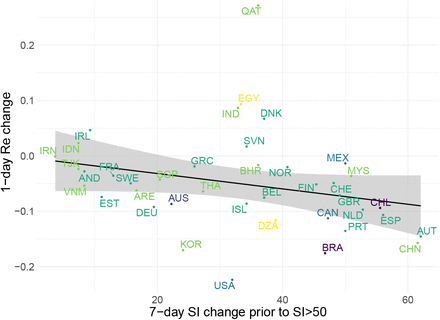
(a) Estimated Re (top) and government stringency index (bottom) for India, South Africa, Switzerland, and the United States of America. (b) Relation between the slope of the Re estimates on tSI50 and the increase in the stringency index over the 7 days prior to tSI50 for 19 European countries. The countries are indicated by their ISO3 country code.
A strong government response is associated with a faster decrease in Re
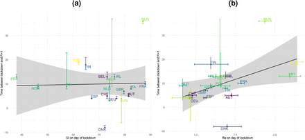
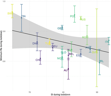
Next, we asked whether the slope of Re on the reference date tSI50 (one-day change) is associated with the decisiveness of the government response, as measured by the change in the stringency index the week prior. In Europe, larger changes in the SI prior to tSI50 were significantly associated with stronger decreases in the estimated Re on the reference date (p = 0.04, adjusted R2 = 0.18, Fig. 3(b); 19 countries). The same trend was found at a global scale, though no longer significant (Fig. S9; 40 countries). However, this does not mean that the SI at lockdown is a predictor for the time until Re is below 1 (p = 0.9, Fig. S10(a)). This time instead was better predicted by the estimated Re on the day of lockdown (p = 0.03, adjusted R2 = 0.2, Fig. S10(b)). Finally, there is no significant association between higher maximum SI during lockdown and a lower minimum Re attained during that time (p = 0.14, Fig. S11).
Insights into continent-specific responses to NPIs
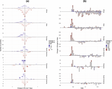
To investigate the association between changes in government stringency and changes in Re in more depth, we extended our analysis until November 10th and included both the implementation and lifting of NPIs (increases and decreases in stringency). For each week and country, we determined whether the stringency index changed, and if so, what the effect was on Re after 7 days. If NPIs are working as expected, increases in stringency should be associated with a decrease in Re and vice versa. We do find this for increases in stringency e.g in Europe (blue bars, Fig. 4a), but decreases in stringency have a more varied effect on Re estimates on all continents (red bars, Fig. 4a). This may be modulated by temporal differences in when NPIs were implemented or lifted (Fig. 4b).
(a) Histogram of the estimated 7-day change in Re following the implementation (blue, above x-axis) or lifting (red, below x-axis) of NPIs in a given week. The height of the bars is given by the number of countries with this observation, coloured by the change in stringency index that week. If NPIs are working as expected, we would expect an increase in stringency (i.e. bars above the x-axis) to be more associated with a decrease in Re (shifted to the left) and bars below the x-axis to be shifted more to the right. Note, scales differ between the continents. (b) Strength of NPI changes through time, coloured by their effect on Re (increase is blue, a decrease red). Here, the height of bars is given by the summed change in the stringency index over all countries that week. If NPIs are working as expected, we would expect bars above the x-axis (i.e. an increase in stringency) to be more red (i.e. associated with a decrease in estimated Re) and bars below the x-axis to be more blue.
For North America, Asia, and Europe, an increase in stringency was significantly more associated with a subsequent reduction in the estimated effective reproductive number Re than a reduction in stringency was (permutation test randomising SI increase/decrease associated with the estimated change in Re, α = 0.05, 6-way Bonferroni correction). For these continents, increases in stringency also resulted in a stronger absolute change than decreases in stringency (permutation test randomising SI increase/decrease associated with the estimated change in Re, α = 0.05, 6-way Bonferroni correction). This suggests that reversing non-pharmaceutical interventions had a very different effect than introducing them. For the continents Africa, South America, and Oceania no significant difference could be detected between the distributions of estimated Re changes after implementation or lifting of NPIs.
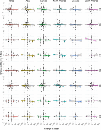
We further repeated this analysis for 8 individual indices that make up the SI compound index separately. Continents differ substantially in which indices showed signal that an increase in stringency was significantly more associated with a subsequent reduction in Re than a reduction in stringency. Four index-continent pairs showed a significant effect: school closing and closing public transport in Europe, cancelling public events in South America, and stay at home requirements in North America (as determined by permutation test randomising SI increase/decrease associated with the estimated change in Re, α = 0.05, 6*8-way Bonferroni correction; Supplementary Table S3). Similar, yet non-significant, trends were observed for some of the other index-continent pairs. We further tested whether there was a linear relationship between the change in stringency of the individual indices and the resulting estimated change in Re (Supplementary Fig. S12, Table S4). The highest R2 values were found for the index-continent pairs also identified in the previous analysis.
3 Discussion
We have developed a pipeline to monitor the effective reproductive number Re of SARS-CoV-2 in near real-time, and validated our estimates with simulations. We showed that the inferred Re curve can be slightly over-smoothed on simulated data, but that this is a necessary compromise given the inherent noisiness and sometimes low quality of real data. Overall, we show that the relative error in the Re estimates is small. In particular, we can detect when Re crosses the critical threshold of 1, which is important to an informed public health response.
During the ongoing SARS-CoV-2 pandemic, Re estimates are of interest to health authorities, politicians, decision makers, the media and the general public. Because of this broad interest and the critical importance of Re estimates, it is crucial to communicate both the results as well as the associated uncertainty and caveats in an open, transparent and accessible way. This is why we display daily updated results on an online dashboard, accessible at https://ibz-shiny.ethz.ch/covid-19-re/. The dashboard shows Re estimates in the form of time series for each included country or region, and a global map containing the latest Re estimates and normalised incidence. For a number of European countries, we also display a timeline of the implementation and lifting of non-pharmaceutical interventions (NPIs). For all countries, we display a timeline of the stringency index of the Blavatnik School of Government.
A unique advantage of the monitoring method we have developed is the parallel use of different types of observation data, all reflecting the same underlying infection process [6]. Wherever we have data of sufficient quality, we estimate Re separately based on confirmed cases, hospitalisations and death reports. The advantages and disadvantages of the different observation types are discussed in the Supplementary discussion 6.1. Comparing estimates from several types of data is a powerful way to evaluate the sensitivity of the results to the type of observations they were derived from. More generally, the method would be applicable to any other type of incidence data, such as admissions to intensive care units or excess death data. The potential limitations of our Re estimation method are discussed in detail in the Supplementary Discussion 6.2.
The decision to implement, remove or otherwise adjust measures aimed at infection control will be informed by epidemiological, social and economic factors [30]. We can aid this decision making process by investigating the association between adjustments of public-health measures and the estimated Re.
The merits of nation-wide lockdowns have been heavily discussed, both in the scientific literature as well as in the public sphere [8, 25, 23, 24, 31]. In particular, analyses showing that Re estimates had dropped below 1 before the strictest measures were enforced were frequently used to claim that a lockdown was not necessary [31]. We showed that this argumentation is flawed: for 17 out of 20 European countries, we found that the estimated Re was significantly above 1 prior to the lockdown in spring.
For this first epidemic wave, we further investigated the link between the strength of NPIs implemented and the concurrent decrease of Re. There was a trend that countries with a strong increase in stringency prior to the reference date tSI50 saw a faster decrease in pathogen transmission on that day. However, this analysis focused only on the estimated one-day change in Re around the onset of the lockdown. We did not find that the strength of the government response significantly determined the time it takes to bring Re < 1, nor the value of Re during a lockdown. To investigate these points conclusively, further analyses are needed that are beyond the scope of this manuscript.
Extending our analysis to data up until Nov. 10, we find differences between continents in the effect of NPIs on Re. This could reflect differences in the speed with which lockdowns were put into practice [26], the de-facto lockdown stringency, or socio-cultural aspects [30, 32]. It is often argued that, especially in countries with a large informal business sector, there may be a difference between the official containment measures and those adhered to or implemented de-facto [32]. However, for continents where we find no significant effect of NPI implementation, this could also be because the majority of NPIs were implemented at a time for which we could not estimate changes in Re. Many African countries implemented early and strict government responses, often prior to the first detected cases. These are thought to have delayed the virus in establishing a foothold on the continent [32]. Since we cannot estimate Re without cases, such early response would not be seen to reduce Re in our analyses.
Importantly, our analysis suggests that reversing non-pharmaceutical interventions had a very different effect than introducing them. This could be because the situation is not fully reverted: due to increased public awareness, testing, contact tracing, and quarantine measures still in place. In addition, the epidemic situation - in terms of number of infected individuals - is likely different when measures are implemented or lifted.
Our analysis could be confounded by other economic, social, and psychological factors motivating the implementation or release of measures. With the current stringency measures we can not account for diversity in adherence to NPIs across geographic regions and through time. Cultural norms, defiance towards public authorities, “lockdown fatigue”, and economic pressures are all among the factors that may determine whether NPIs are in fact adhered to. In addition, there is increasing evidence that weather may be a factor influencing Re through its effect on people’s behaviour as well as properties of the virus [33]. In the future, our tools to quantify Re could be used to explore associations of these many factors with Re, with the aim of identifying minimal sets of factors ensuring an Re < 1 for particular locations.
Data Availability
All code and data is publicly available except for the line list of Swiss cases provided by the Federal Office of Public Health (we could not obtain permission to publish this data)
3.1 Author contributions
J.S.H, J.S, S.B, T.S designed research; J.S.H, J.S, D.C.A, R.A.N contributed new reagents or analytic tools; J.S.H, J.S performed research; J.S.H, J.S analyzed data; and J.S.H, J.S wrote the paper. All authors critically reviewed and approved the paper.
4 Materials and Methods
4.1 EpiEstim
The method presented here builds upon the Re estimation method developed by Cori et al. [12], implemented in the EpiEstim R package. This method estimates Re(t) from a time series of infection incidence, we summarise its details below.
Disease transmission is modelled with a Poisson process. At time t, an individual infected at time t −s causes new infections at a rate Re(t) ·ws, where ws is the value of the infectivity profile s days after infection. The infectivity profile sums to 1, and can be approximated by the serial interval distribution [12]. The expected infection incidence It at time t is thus:
 and the likelihood of the incidence It is given by:


The Re(t) inference is performed in a Bayesian framework, and an analytical solution can be derived for the posterior distribution of Re(t) (see [12]; Web Appendix 1). We choose a gamma distributed prior on Re(t) with mean 1, and standard deviation 5.
4.2 Deconvolution
To recover the non-observed time series of infection incidence, we deconvolve the observed time series of COVID-19 case incidence with a delay distribution specific to the type of case detection (case confirmation, hospital admission, death).
We extended the deconvolution method of Goldstein et al. [14], which is itself an adaptation of the Richardson-Lucy algorithm. Formally, the deconvolution infers an infection incidence time series (λ1, …, λN) from a time series of observed cases (DK, …, DN), with K ≥ 1. Di indicates the number of observed cases on day i. Let  be the probability that an infection on day j takes l days to be detected. For any k < 0 and any,
  . If no line list data is available
  , and no time-variation of the delay distribution is assumed. Let qj be the probability that an infection that occurred on day j is observed during the time-window of observations, between days K and N. Then:

Let Ei be the expected number of observed cases on day i, for a given infection incidence (λk):

The Richardson-Lucy algorithm uses expectation maximisation to find a final infection incidence estimate, which has the highest likelihood of explaining the observed case time series. To do so, it starts from an initial guess of the infection incidence time series  , and updates the estimate in each iteration n according to the following formula:

The iteration proceeds until a termination criterion is reached. Here, we follow Goldstein et al. and iterate until the χ2 statistic drops below 1 [14], or 100 iterations have been reached:

Convergence is typically fast and the stopping criterion based on the χ2 statistic is reached in a few iterations. Due to the smoothing prior to deconvolution, this was the case for nearly all empirical data we analyzed. In some cases, e.g. when the observed incidence is very noisy, convergence can be slower and the threshold of 100 iterations can be reached. For 4/170 countries, convergence was not reached in 100 iterations: China, Ecuador, Equatorial Guinea and Peru all showed strong spikes in reporting which obstructed the deconvolution.
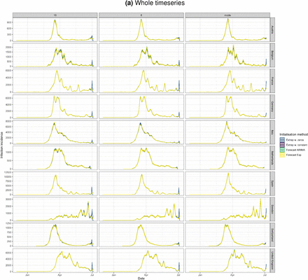
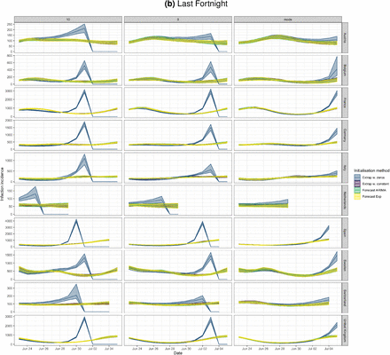
For the initial estimate of the incidence time series Λ0, we shift the observation time series backwards in time by the mode of the delay distribution µ [14]. However, this leaves a gap of unspecified values at the start and end of the time series Λ0. Contrary to Goldstein et al., we augment the shifted time series with the first observed value (DK) on the left, and with the last observed value (DN) on the right, to avoid initialising with a zero-value anywhere. If a day is initialised with zero incidence, it will also have zero incidence in the final estimate (compare equation 6), which would be a potential source of bias. We have compared several ways to pad the shifted observed time series for the initialisation step, and determined that augmentation with non-zero integers equal to the edge values is enough for the deconvolution to converge to the true distribution (see Supplementary Fig. S13).
We note that this Richardson-Lucy deconvolution algorithm accounts for ‘right truncation’, i.e. not all infections that have occurred are observed within the given observation time window (due to delay until symptoms/reporting), through the qj indices.
Use of line list data
When a line list is available, the time variation of delays between symptom onset and observation can be taken into account directly during the deconvolution step. This leads us to perform the deconvolution in two separate steps: first with the time-varying empirical onset-to-observation distributions, and then with the constant-through-time incubation period distribution. For those cases where symptom onset data is available, we only deconvolve with the incubation period distribution.
The  time-varying delay distributions from onset of symptoms to observation are determined as follows: for each date j, at least 300 of the most recent recorded delays between symptom onset and observation, with onset date before j, are taken into account. To avoid biases caused by the intensity of testing and reporting varying throughout the week, recorded delays are included in full weeks going in the past, until at least 300 delays are included.
As the incidence data is right-truncated, we have to fix the reporting delay distributions  at some point, or they would be downward biased for infection dates close to the present. Let
  be the overall empirical delay distribution (aggregated over the entire window of observations) and n the 99th percentile of this distribution (n is the smallest integer for which
  . For all infection dates z such that M −z < n, M being the index of the last available data point, we fix
  to be equal to
 .
.
4.3 Noise and uncertainty in the case observations
To reduce the influence of weekly patterns in case reporting data, as well as reporting irregularities, we smooth the observed incidence data prior to deconvolution. To smooth the incidence data, we use local polynomial regression fitting (LOESS) with 1st order polynomials and tricubic weights. The smoothing parameter alpha is set such that we always include 21 days of data in the local neighbourhood of each point. At the edges, the weights drop to 0 and less points are taken into account in total [34]. After smoothing, we normalise to the original total number of cases.
To reflect uncertainty in the observation process, we bootstrap the observed incidence data 50 times, prior to smoothing, deconvolution, and Re estimation. The bootstrapping process here consists of sampling reported cases with replacement from the original case data (with equal probability per case), until a resampled time series with the same number of cases as the original one is obtained. This likely underestimates the total uncertainty because it does not take into account that some cases may be correlated, e.g. by belonging to the same transmission chain. A common way to circumvent this problem would be to use a (moving) block bootstrap method. We are working to implement this into our pipeline.
The Re estimate reported for day T summarises the average estimated Re over a 3-day period ending on day T. We report the median of the 50 Re posterior distributions obtained, as well as the median of the 95% uncertainty interval boundaries. In addition, we provide step-wise estimates of Re. In this step-wise analysis, Re is assumed to be constant on a number of intervals spanning the entire epidemic time window. These intervals are bounded by dates at which public health interventions were implemented, altered, or lifted.
4.4 Data
We gathered case incidence data directly from public health authorities. Whenever accessible, we rely on data from local authorities. Otherwise, we default to the data of the European Centre for Disease Control (ECDC) [35]. A table summarising the incidence data sources is available in Supplementary File S1. Information on the start and end of interventions, or major changes in testing policy, were obtained from media reports and the websites of public health authorities. The stringency index of the Blavatnik School of Government was accessed from their publicly available github repository [29].
We parametrised the discretised infectivity profile ws using COVID-19 serial interval estimates from the literature [36], i.e. a gamma distribution with a mean of 4.8 days, and a standard deviation (SD) of 2.3 days. For a review of serial interval estimates published in the literature, see Griffin et al. [37]. The incubation period is parametrised by a gamma distribution with mean 5.3 days and SD 3.2 days-[38]. For countries for which we do not have access to line list data, i.e. all except Switzerland, Germany and Hong Kong at the time of writing, we assume delays from symptom onset to observation to be gamma-distributed, see table 2 for parameters.
For Switzerland, Germany and Hong Kong, we use line lists to build time-varying empirical distributions on delays between symptom onset and case confirmation, hospitalisation or death. During the deconvolution step we use the empirical delay distribution of the last 300 recorded cases prior to the infection date. Moreover, for the fraction of cases for which the date of onset of symptoms is known, we use the onset date directly instead of deconvolving a delay from onset to reporting, allowing for more precise estimation of the infection date. For Switzerland, line lists contain information on which cases were infected abroad. By considering imported cases and locally-transmitted cases separately in the deconvolution step, we obtain two separate time series, one for local infections and one for imported infections.
4.5 Simulations
In the simulations, we first simulate a time series of infections and corresponding case observations from a specified piecewise linear Re trajectory. Then, we estimate Re from these observations using our method: deconvolution to infer the infection time series, followed by EpiEstim to estimate Re.
To assess a range of scenarios, we parametrise Re as a piecewise linear trajectory, where we fix the plateau values for Re and the time-points at which the trajectory changes slope. Assuming I0 infected individuals on the first day, the infection incidence is simulated forward in time, using the Re time series and the discretised serial interval for SARS-CoV-2 [36] (see [12]; Web Appendix 11). These simulated infections are convolved with the observation type-specific delay distribution [38] to obtain the raw observation time series. In the case of time-varying delay distributions, we assume the mean of the delay distribution decreases by a fixed amount (1/20) each day, to a minimum of 2 days (e.g. for the confirmed cases this results in a range from 4.5 to 2). When estimating with a time-varying delay distribution, we draw observations from the true distributions, similar to line list information recorded by public health authorities. To assess the added value of the deconvolution method, we compare against a method where we estimate the infection time series by shifting the observations back by the mean of the delay distribution (termed ‘fixed shift method’).
To obtain the final observation time series we can add either weekly or daily sources of noise. In the case of weekly noise, we reduce the number of cases on the weekend to a fraction f of the simulated number, and add the subtracted cases to the following Monday and Tuesday instead. In the case of daily noise, we add multiplicative Gaussian noise with mean 1 and a set standard deviation on every day of the time series. If both sources of noise are chosen, the weekly noise is applied first.
Performance metrics
To quantify the performance of our method on the simulated scenarios, we employ 5 metrics. The normalised root mean square error (RMSE) is given by:
 where
where  indicates the mean true Re, N the length of the time series,
  the estimated Re and Rj the true Re at time j. The relative error of the slope of the initial decrease (Slope error) is determined by comparing the slope of the true and estimated Re between the time of the end of the first Re plateau
  and the start of the second plateau
  . The date of the R = 1 crossing (R = 1 difference) is determined by the number of days difference between when the true Re crosses the threshold of R = 1 and our Re point estimate does so. The fraction of correct above or below 1 estimation (Correct R > 1/R < 1) is determined as the fraction of the time series where we correctly infer that Re is significantly above or below 1. Time points where the confidence interval includes values both above and below 1 are excluded from the calculation. The empirical coverage (Coverage) indicates the fraction of the time series for which our confidence interval includes the true Re value.
4.6 Implementation and method availability
Daily updated results of our method on global COVID-19 data are available online on https://ibz-shiny.ethz.ch/covid-19-re/. The source code of this pipeline is openly accessible (see https://github.com/covid-19-Re/dailyR). We are also continuously updating our data sources, and welcome anyone who wishes to share quality data for a particular region or country (please contact the authors, or raise an issue on the Github repository of this project at https://github.com/covid-19-Re/shiny-dailyRe).
6 Supplementary Discussion
6.1 Observation types and the influence of testing
Here, we briefly discuss the benefits and potential biases of the three types of observations we used. The most commonly used proxy for infection incidence is the incidence of confirmed cases. It is the least indirect way of observing infection events. However, it generally assumes that (i) the proportion of infected individuals that is tested, and (ii) the distribution of the delay between infection and testing are constant through time. Unfortunately, these assumptions do not generally hold.
As long as the sampling proportion is constant throughout the considered time period, the Re estimates of EpiEstim are not affected by under-sampling [12]. During the SARS-CoV-2 epidemic, many countries initially restricted testing to only severe cases, before switching to a more extensive testing effort after curbing the first epidemic wave and ramping up testing capacity [41]. Changes in testing strategy as well as bottlenecks in testing capacity result in a varying fraction of infected individuals that are confirmed positive, but also in the delay between infection and test confirmation. This can bias the Re estimate, as it will attribute an increase/decrease in case numbers between consecutive time points to a change in infection incidence, rather than a change in testing.
However, it is important to note that the ‘memory’ inherent in the Re estimate is dictated by the serial interval ws. An event at time t which changes the proportion of true infection incidence observed per day, e.g. a change in testing policy, will bias the Re estimate for the number of days needed to reach the 95% of ws (compare Materials and Methods, equation 1). We do not observe the infection incidence directly, but if the deconvolution is assumed to be perfect, the intuition for the number of days of biased Re estimates still holds.
It is further possible to investigate the influence of testing intensity, by applying the Re estimation method separately to a case incidence time series which is adjusted for the intensity of the testing effort. We have added this analysis to our online dashboard (where we show the number of confirmed cases / number of tests, normalised by the mean number of tests). However, one should note that such a normalisation does not take into account that the probability of test positivity might also change with the number of tests (e.g. by prioritising likely cases at low numbers of tests).
In contrast, the incidence of hospital admittance and deaths are likely based primarily on the severity of the symptoms, and mostly unaffected by changes in testing strategies, or the magnitude of the epidemic. This makes them valuable complementary observations of infection events [14]. However, also here biases can occur. First, only a small fraction of all infections results in hospitalisation or death (a recent meta-analysis found an average infection fatality ratio for SARS-CoV-2 of 0.68% [42]). This fraction varies with the risk group of the infected population [42, 43, 44, 45], introducing potential biases in Re estimations when outbreaks occur in particularly age-stratified settings. Second, if a country’s health infrastructure becomes overburdened and hospitals are forced to triage or delay admission, we expect the fraction of hospital admissions to decrease, and deaths to increase. Third, the likelihood to die from an infection may change through time as new treatment strategies are developed. Additionally, guidelines used to record COVID-19 as the cause of death have changed through time for some countries [46]. Lastly, the delay between infection and hospitalisation or death is expected to be longer than the delay until case confirmation, with the result that these Re estimates are less timely. One should note that these observation type specific biases could also be seen as a source of information. The types simply describe a different epidemic if very structured population with highly different mortality rates are captured (e.g. elderly homes).
6.2 Method Limitations
The Re estimation method we present in the main text relies on several assumptions. Here we highlight the limitations that occur when these assumptions are violated.
First, the geographical scale of the Re estimates is determined by the incidence data itself. The Re calculated for a country represents an average, summarised across multiple local epidemics unfolding in different regions. Re values need not be identical in different local epidemics across a country or administrative region. In particular, in times of very low pathogen transmission, single super-spreading events can significantly increase the estimated Re of the entire country [47].
Second, in our deconvolution step we account for an incubation period and a delay from symptom onset to case observation. Implicitly, we thus assume that all reported cases come from symptomatic individuals. This is certainly true for hospitalised and deceased patients, but does not have to hold for all confirmed cases. Similar to the testing intensity (discussed in Section 6.1), this would not bias our estimates as long as the fraction of asymptomatic or presymptomatic individuals is constant through time. However, the fraction of asymptomatic individuals could vary with the population structure and age-stratification. The fraction of tested presymptomatic individuals could vary with the testing strategy and the intensity of the testing effort.
Third, in our current analysis we assume a single serial interval distribution for all geographic locations and all times. However, behaviour, population contact structure, and cultural differences in dealing with infection symptoms, will cause geographic and temporal variations in the serial interval. In particular, the implementation of non-pharmaceutical interventions can significantly shorten the serial interval [7]. Misspecification of the generation interval will be most pronounced for Re values further away from one [13].
Lastly, our estimates of the effective reproductive number Re are subject to changes in data reporting. There are frequent changes in the way in which public health offices update their observed incidence data: the amount of variables shared (e.g. Brasil, the UK excluded testing information), their frequency (e.g. Swiss cantons moved to weekly data updates when daily numbers became low), the amount of consolidation (i.e. how much values reported for a given day change in subsequent days), and what constitutes a COVID-19 case [46]. These variables have all changed during the epidemic, frequently in response to political pressure or the magnitude of the local epidemic and the resulting workload at the public health offices [46]. This affects the timeliness of our estimates, and can cause the estimated Re to change a bit between days.
7 Supplementary Methods
Discretisation of delay distributions
When approximating delay distributions by gamma distributions, we discretise these in the following fashion:
 where f is either the probability density function (p.d.f) of the gamma-distributed delay distribution, or the p.d.f of the sum of two independent gamma-distributed delay distributions. The former applies when line list data is available, and the observed data is deconvolved with the gamma-distributed incubation period separately from the empirical delay distribution of symptom onset to observation. The latter applies whenever the observed case data is jointly deconvolved with the incubation period and delay between symptom onset and observation.
Because the probability density function of a sum of two independent gamma distributions does not admit a simple form in the general case, in practice we approximate the p.d.f by drawing a million independent pairs of samples, one from each gamma distribution, summing the pairs, and computing the empirical cumulative distribution function of the sampled distribution.
8 Supplementary Materials
8.1 Supplementary Simulations
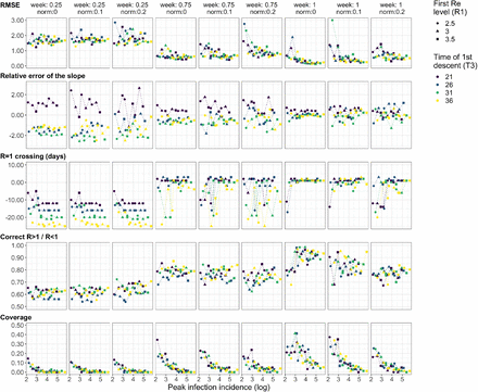
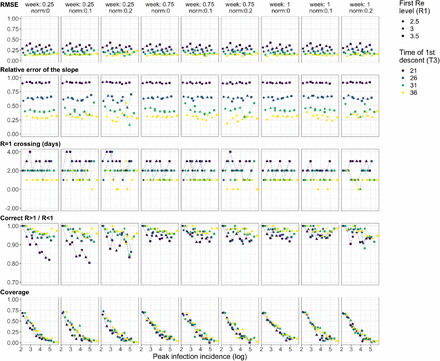
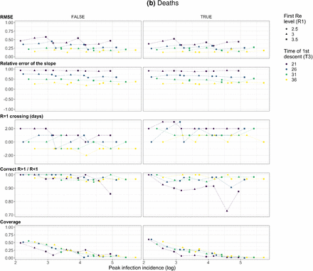
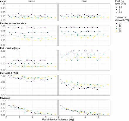
The R1 (point shape), t3 (point colour), and I0 were varied, all other parameters kept constant (see Materials and Methods 4.5). Three plateaus were used, with R2 = 0.5, R3 = 1.2. The columns indicate different combinations noise: weekly noise (‘week’) reduces the number of cases on the weekend to a fraction f and redistributes these to Monday and Tuesday (f = 1 is the weakest noise), and daily noise (‘norm’) which refers to multiplicative Gaussian noise with mean 1 and a set standard deviation sd on every day of the time series (sd = 0 is weakest).
The R1 (point shape), t3 (point colour), and I0 were varied, all other parameters kept constant (see Methods 4.5). Three plateaus were used, with R2 = 0.5, R3 = 1.2. The columns indicate different combinations noise: weekly noise (‘week’) reduces the number of cases on the weekend to a fraction f and redistributes these to Monday and Tuesday (f = 1 is the weakest noise), and daily noise (‘norm’) which refers to multiplicative Gaussian noise with mean 1 and a set standard deviation sd on every day of the time series (sd = 0 is weakest).
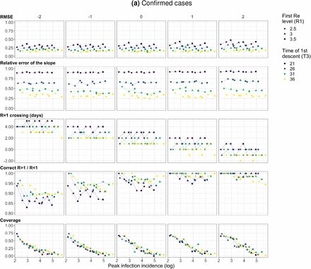
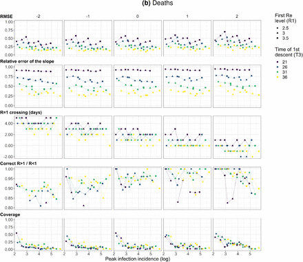
We changed the mean of the delay distribution (5.5 for symptom-onset to case confirmation, 15.0 for symptom-onset to death) by the numbers above the columns. The R1 (point shape), t3 (point colour), and I0 were varied, all other parameters kept constant (see Materials and Methods 4.5). The observations were smoothed and no noise was added. Three plateaus were used, with R2 = 0.5, R3 = 1.2. No noise was added to the observations.
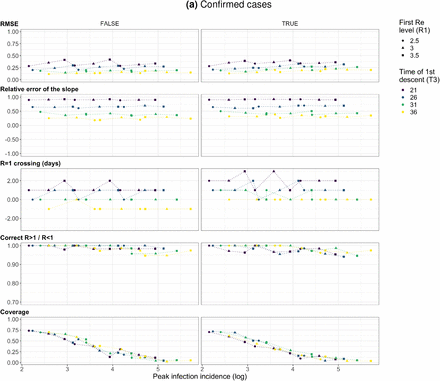
The observations were simulated with time-varying delay distributions (see Materials and Methods, section on simulations), and then estimated with (right column) or without (left column) taking the time-varying distributions into account. The R1 (point shape), t3 (point colour), and I0 were varied, all other parameters kept constant. The observations were smoothed and no noise was added. Three plateaus were used, with R2 = 0.5, R3 = 1.2.
In case of the fixed shift method the observations are shifted back by the mean of the delay distribution. For both methods the observations are bootstrapped in the same way, leading to similar width of the confidence intervals. The R1 (point shape), t3 (point colour), and I0 were varied, all other parameters kept constant (see Materials and Methods 4.5). The observations were smoothed and no noise was added. Three plateaus were used, with R2 = 0.5, R3 = 1.2.
8.2 Switzerland specific results
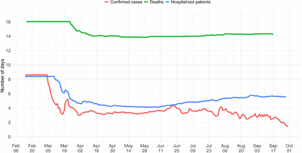
For each date, the mean is taken over the last 300 reports with known symptom onset date, based on line list data from the FOPH. For early dates, before 300 reports are available, the mean is taken over the first 300 reports.
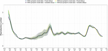
The comparison is based on time series of confirmed cases in Switzerland, from line list data provided by the FOPH. Both the inclusion of known symptom onset dates and of the time-variability of reporting delay distributions have an effect on the Re estimates, in particular for early estimates in this case.
8.3 R = 1 crossings
The comparison is based on time series of confirmed cases in Switzerland, from line list data provided by the FOPH. The analysis without imports is unbiased if the number of imports equals the number of exports. Since the analysis accounting for imports is not accounting for exports, the results are a lower limit for the effective reproductive number.
Based on news reports, we determined when a country implemented stay-at-home orders (a ‘lockdown’). Using our method we determined when the Re estimate and its confidence intervals first dropped below 1. Based on our Re estimates for confirmed cases, only two countries that implemented a nationwide lockdown (Denmark, Slovenia) had confidence intervals that included or were below one before a nationwide lockdown was implemented. For Re estimates based on COVID-19 deaths, there are also two, but different ones (the Netherlands, Poland).
News and public resources used to determine when a country implemented the first non-pharmaceutical interventions, and a nationwide lockdown.
SI 50 analysis Reference date: first day the stringency index exceeded 50 (SI > 50).
The 39 included countries: Algeria, Andorra(*), Australia, Austria, Bahrain, Belgium, Brazil, Canada, Chile, China, Denmark, Egypt, Estonia, Finland, France, Germany, Greece, Iceland, India, Indonesia, Iran, Ireland(*), South Korea(*), Malaysia, Mexico, Netherlands, Norway, Portugal, Qatar, Singapore, Slovenia, Spain, Switzerland, Tajikistan, Thailand, United Arab Emirates, United Kingdom, United States of America, Vietnam.
The star indicates the country was not included in the ΔSI analysis.
For 34/39 countries the Re estimate was above one prior to the reference date, and significantly so for 28/39. The countries that reached Re < 1 prior to the reference date were Andorra (15 days prior), Australia (1 day prior), Denmark (3 days prior), Qatar (5 days prior), and Vietnam (2 days prior).
ΔSI analysis Reference date: date of the biggest 7-day increase in the SI.
The 50 included countries: Algeria, Australia, Austria, Bahrain, Belarus(*), Belgium, Brazil, Canada, Chile, China, Colombia(*), Croatia(*), Czech Republic(*), Denmark, Egypt, Estonia, Finland, France, Germany, Greece, Iceland, India, Indonesia, Iran, Israel(*), Japan(*), Lebanon(*), Malaysia, Mexico, Netherlands, New Zealand(*), Norway, Pakistan(*), Philippines(*), Portugal, Qatar, Russia(*), Serbia(*), Singapore, Slovenia, Spain, Sweden(*), Switzerland, Tajikistan, Thailand, Turkey(*), United Arab Emirates, United Kingdom, United States of America, Vietnam.
The star indicates the country was not included in the SI50 analysis.
For 44/50 countries the Re estimate was above one prior to the reference date, and significantly so for 36/50. The countries that reached Re < 1 prior to the reference date were Australia (2 days prior), Denmark (4 days prior), New Zealand (2 days prior), Qatar (6 days prior), Tajikistan (17 days prior), and Vietnam (9 days prior).
Relation between the slope of the Re estimates on tSI50 and the increase in the stringency index in the 7 days prior to tSI50. Countries are indicated by their ISO3 country code, colours represent continents.
8.4 Implementation/Lifting of individual NPIs
8.5 Sensitivity of the deconvolution to initial conditions
(a) The stringency index on the day of lockdown is not a good predictor for the number of days it will take for Re < 1 (p = 0.9). (b) The Re estimate on the day of lockdown is significantly associated with the number of days it will take for Re < 1 (p = 0.03, adjusted R2 = 0.2). The regression analysis used the Re point estimate for each country. The uncertainties shown in the plot were not used for this analysis. Countries are the same as in table 1, and indicated by their ISO3 country code.
This trend is not significant (p = 0.14). Lockdown here refers to the period of constant, maximum stringency during the first wave in Europe (April 2020). There is substantial variation in the duration of the lockdown, and the number of days after the start of the lockdown that the minimum Re was reached. The regression analysis used the Re point estimate for each country. The uncertainties shown in the plot were not used for this analysis. Countries are the same as in table 1, and indicated by their ISO3 country code.
Significance was determined by permutation test for each index separately, with significance threshold α = 0.05, and corrected for 48-way hypothesis testing.
Significance was determined with significance threshold α = 0.05, and corrected for 48-way hypothesis testing.
The rows C1-C8 refer to different stringency indices (see table S4).
Panel (b) shows the last fortnight of panel (a). Confidence intervals are computed on 20 bootstraps of the original time series. The columns represent a shift by 10 days, 8 days, or the mode of the delay distribution (7 days). The rows show ten countries in our dataset. It is clear that augmenting both ends with zeros can lead to spurious increases in incidence towards the present (blue curves). Augmenting with a constant non-zero integer (purple), forecasting with an ARIMA model (green), and forecasting with an exponential model (yellow), all perform similarly.
Acknowledgements
We thank the Federal Office of Public Health Switzerland for access to their line list data, and members of the modelling group of the Swiss National Covid-19 science task force for helpful discussions. We thank Marloes Maathuis for her feedback to the paper, discussions, and follow-up work on the bootstrapping methods together with Jinzhou Li. We thank Jūlija Pecčerska for her help in finding governmental datasets on COVID-19. JSH was funded by the NRP72 SNF grant (407240-167121) awarded to SB and TS. SB and TS thank ETH Zurich for funding.


