Abstract
Genome-wide association studies seek to attribute disease risk to DNA regions and facilitate subject-specific prediction and patient stratification. For later-life disease, inference from case-control studies is hampered by the uncertainty that control group subjects might later be diagnosed. Time-to-event analysis treats controls as right-censored, making no additional assumptions about future disease occurrence and representing a more sound conceptual alternative for more accurate inference. Here, using data on 11 common cancers from the UK and Estonian Biobank studies, we provide empirical evidence that discovery and genomic prediction are greatly improved by analysing age-at-diagnosis, compared to a case-control model of association. We replicate previous findings from large-scale case-control studies and find an additional 59 previously unreported independent genomic regions, out of which 16 replicated in independent data (an increase of 18% and 6% over current findings). Our novel discoveries provide new insights into underlying cancer pathways, and our model yields a better understanding of the polygenicity and genetic architecture of the 11 tumours. We find that heritable germline genetic variation plays a vital role in cancer occurrence, with risk attributable to many thousands of underlying genomic regions. Finally, we show that Bayesian modelling strategies utilising time-to-event data increase prediction accuracy. As sample size increases, incorporating time-to-event data should be commonplace, improving case-control studies by using richer information about the disease process.
Introduction
Cancer has broad medical importance and a high global health burden, with 19.3 million new cancer cases and almost 10 million cancer deaths occurring in 2020 [1]. Genome-wide association studies (GWAS) aim to attribute risk to regions of the DNA [2] and facilitate polygenic risk score (PRS) calculation [3] to predict subject-specific risk, which may then enable targeted and improved healthcare [4–6]. There is currently evidence for only 450 genomic regions associated with increased risk of 18 common cancers [2], despite recent results showing significant non-zero heritability across a range of cancer occurrences [7]. Current PRS calculated from these findings stratify risk for several cancers, including breast, colon, and prostate cancer, but often add negligible additional predictive information compared to existing non-genomic predictors [8]. Increasing sample size yields increased statistical power for discovery, with extensive recent case-control studies for breast cancer [9], prostate cancer [10, 11], ovarian cancer [12], or testicular cancer [13] showing improved results, but this remains a challenging endeavour. Biobanks provide an additional resource, essential for modern-day medical genetics; however, individuals within these studies have not all reached old age and the number of cancer cases is not high, with recent studies combining biobank cohorts for 18 cancer types [7] to limited effect.
Increased statistical power can also stem from tailored modelling choices, and one factor behind limited predictive performance could be the choice of the genome-wide analysis method. Although most association studies use methods that account for the impact of other genetic regions (fastGWA [14], GMRM [15], BoltLMM [16], REGENIE [17]), it is sometimes still preferred to resort to the basic association testing. In addition, most genome-wide analyses have been performed using a case-control phenotype rather than utilising the cancer diagnosis age as a phenotype, and there is some evidence that analysing data using time-to-event informed methods can have more power for detecting associations [18–21].
Here, we provide empirical evidence using data on 11 common tumours from the UK and Estonian Biobank studies that GWAS discovery and genomic prediction are greatly improved by analysing age-at-diagnosis, compared to a case-control model of association. We extend our recently presented BayesW approach [20], a Bayesian modelling framework that enables joint effect size estimation for time-to-event data, to provide marginal leave-one-chromosome-out mixed-linear age-at-onset adjusted association estimates, in contrast to using Cox mixed model [22] or age-at-onset informed genomic reconstruction of the phenotype [21]. We focus on a re-analysis in the UK Biobank data alone, and we replicate previous findings from large-scale case-control GWAS and find an additional 59 previously unreported independent genomic regions, out of which 16 replicated in independent data (a respective increase of 18% and 6% over current findings). Our novel discoveries provide new insights into underlying cancer pathways, and our model yields a better understanding of the polygenicity and genetic architecture of the 11 tumours. We find substantial SNP-heritability, implying that heritable germline genetic variation plays a vital role in cancer occurrence, with risk attributable to many thousands of underlying genomic regions. Finally, we show that Bayesian modelling strategies that utilise time-to-event data give increased prediction accuracy for all analysed tumours and suggest clinically relevant discrimination rules within the Estonian Biobank study. We argue that it is possible to use existing data more thoughtfully and that a re-analysis of case-control study data exploiting age-at-onset information will lead to novel discoveries and enhanced genomic prediction.
Results
Novel and replicated associations
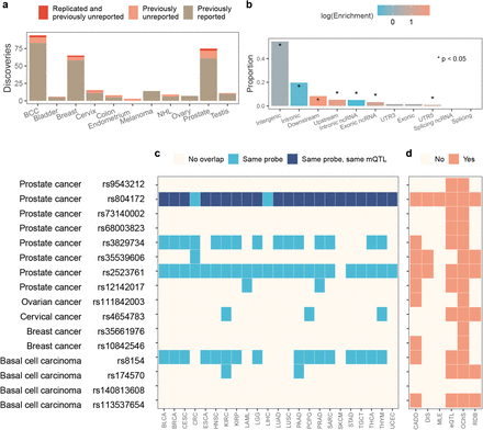
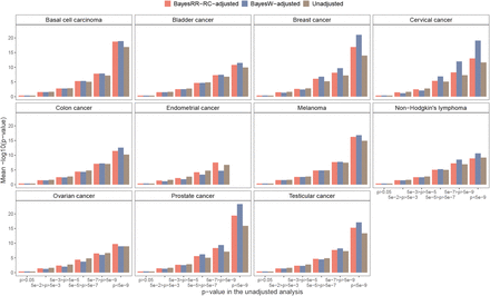
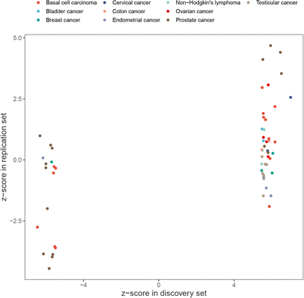
We analysed data from the UK Biobank on the timing or occurrence of diagnosis of 11 different tumours (see Supplementary Information) using 458,747 individuals of European ancestry and a very weakly LD pruned set of 2,174,071 SNP markers (see Methods and descriptive statistics in Table S1). We present a mixed-linear age-at-onset adjusted association model that mimics the behaviour of recently developed leaving one chromosome out (LOCO) linear mixed models [15, 17] and uses age-at-diagnosis information (GMRM-BayesW, see Methods). We compare the results obtained to a recently proposed more classical case-control information mixed-linear association model that uses the same prior structure for the LOCO adjustment but no age-at-onset information (GMRM-BayesRR-RC [15]). We find that this approach of adjusting the phenotypes with either BayesW or BayesRR-RC predictors results in enhanced statistical power (Figure S1), with GMRM-BayesW resulting in higher power gain as compared to GMRM-BayesRR-RC for most cancer sites. Applying GMRM-BayesW or GMRM-BayesRR-RC to the UK Biobank data, we replicate previously reported findings, with 266 previously identified significant independent trait-marker associations at p < 5 · 10−8 (Supplementary data). We also find an additional 59 independent previously unreported variants significant at p < 5 · 10−8, of which 16 replicate in independent data of either the Estonian Biobank or previous non-UK Biobank case-control studies (Figure 1a, Table 1, see Methods). The replication analysis demonstrates that the z-scores for 59 previously unreported associations are correlated between the replication and discovery data sets (Fisher’s exact test for z-score sign p = 0.002, Supplementary figure S3). Furthermore, we observe that the 59 previously undiscovered variants had small but not genome-wide significant p-values in the unadjusted analysis (see Methods), and using GMRM-BayesRR-RC or GMRM-BayesW reduced their p-values below a genome-wide significance threshold (Table S3). We discover novel or replicate previous discoveries slightly better when we account for age-at-onset as compared to the case-control model with 83% and 78% of the markers discovered, respectively, especially for traits that have higher case counts such as breast or prostate cancer (Figure S2).
Mixed-linear association model results were LD clumped such that the index SNPs would have a p-value below 5 10−8 and SNPs could be added to a clump if they were 1Mb from the index SNP, they were correlated with r2 > 0.05 and they were nominally significant (p < 0.05). We then used the COJO method from the GCTA software (see Methods) to find clumps with independent signals by conducting stepwise selection of index SNPs in 1Mb window and we considered SNPs independent if they had a p-value below 5 · 10−8 in the joint model. To determine novelty, we first removed all markers that were significantly associated in the unadjusted model (eq. 3). We then removed all the markers that had a correlation of r2 > 0.1 with a marker that had been previously found associated with a cancer of interest using GWAS Catalog (published until July 2021) and LDtrait tool with the British in England and Scotland population. We then again used COJO to condition the remaining markers on the previously identified associations for each cancer of interest and SNPs that did not fall below 5 · 10−8 in the joint model were eliminated. For the remaining SNPs, we conducted an additional literature review using Phenoscanner database (see Methods) to find any previous associations with variants of interest or variants in LD. The remaining candidates of novel associations were concatenated across GMRM-BayesW or GMRM-BayesRR-RC adjusted analyses and then replicated in the largest available studies conducted for each specific cancer type and the Estonian Biobank. Replication was defined as Benjamini-Hochberg corrected p-value being lower than 0.05 and the direction of the effect size same in both the original analysis and the replication analysis. The column Nearest gene is mapped from the SNP using ANNOVAR software, * in that column denotes intergenic regions.
(a) Count of previously reported discoveries, previously unreported discoveries and previously unreported replicated discoveries using a mixed-linear age-at-onset adjusted association model (GMRM-BayesW) and mixed-linear association model (GMRM-BayesRR-RC). (b) Proportion of SNPs from the novel genetic regions per functional consequences on genes annotated using ANNOVAR; enrichment of functional consequences of SNPs are tested using a two-sided Fisher’s exact test. (c) Overlap of methylation probes affected by SNPs from the novel genetic regions with probes that are differentially methylated across 23 cancers from the Pancan-meQTL database; the probes that are differentially methylated by means of the same SNP are marked dark blue (BLCA - Bladder Urothelial Carcinoma, BRCA - Breast invasive carcinoma, CESC - Cervical squamous cell carcinoma and endocervical adenocarcinoma, CRC - Colon adenocarcinoma + Rectum adenocarcinoma, ESCA - Esophageal carcinoma, HNSC - Head and Neck squamous cell carcinoma, KIRC - Kidney renal clear cell carcinoma, KIRP - Kidney renal papillary cell carcinoma, LAML - Acute Myeloid Leukemia, LGG - Lower Grade Glioma, LIHC - Liver hepatocellular carcinoma, LUAD - Lung adenocarcinoma, LUSC - Lung squamous cell carcinoma, PAAD - Pancreatic adenocarcinoma, PCPG - Pheochromocytoma and Paraganglioma, PRAD - Prostate adenocarcinoma, SARC - Sarcoma, SKCM - Skin Cutaneous Melanoma, STAD - Stomach adenocarcinoma, TGCT - Testicular Germ Cell Tumors, THCA - Thyroid carcinoma, THYM - Thymoma, UCEC - Uterine Corpus Endometrial Carcinoma). (d) Properties of novel replicated genetic regions. CADD - maximum CADD score of the region is above 12.37, DIS - maximum DeepSEA disease impact score (DIS) of the genetic region is above 2, MLE - maximum DeepSEA mean log e-value (MLE) of the region is above 2, eQTL - an SNP from the the genetic region is an eQTL with p-value < 5 · 10−8, OChS - open/active chromatin state (minimum 15-core chromatin score of the lead SNP is less or equal than 7), RDB - minimum RegulomeDB category of the genetic region is 1 or 2.
To map novel associations to functional annotations, we conducted a number of follow-up analyses. SNPs from the previously unreported 16 genomic regions (lead SNPs and those in LD r2 > 0.6, see Methods) lie predominantly in intergenic parts of the genome, with slightly more enrichment than the reference population (enrichment 1.2, p = 5.0 · 10−5). We observe substantially higher enrichment in downstream (7.4, p = 4.3 · 10−21) and upstream (5.0, p = 2.4 · 10−10) regions (the respective values for all significant SNPs are 1.5, p = 6.9 · 10−9 and 1.7, p = 5.4 · 10−14) (Figure 1b). Majority of SNPs from these novel regions could be linked to regulatory variation. Namely, 11 out of 16 genomic regions contain expression quantitative trait loci (eQTLs) (maximum p < 1.8 · 10−20 from FUMA eQTL mapping, see Methods); 6 novel regions have SNPs that fall into RegulomeDB categories [23] that are likely to affect binding, or are linked to expressions of a gene target (Figure 1d). In addition, 5 novel genetic regions include methylation QTLs (mQTLs) associated with other cancers from the Pancan-meQTL database [24]. Moreover, 15 out of 16 novel genomic regions are in open chromatin state in at least 1 of 127 tissue/cell types predicted by ChromHMM [25] (Figure 1d), while for 7 regions, active chromatin state is the most common (Supplementary data).
We confirmed the regulatory effects of novel regions on a wide range of chromatin features using DeepSEA, a deep learning-based model that predicts chromatin effects of sequence variants and priorities regulatory variants [26, 27]. The DeepSEA functionality score median for SNPs in novel genomic regions is 0.18 and one region (index SNP rs804172, associated with prostate cancer) has maximum mean log e-value (MLE) > 2 (Figure 1d), indicating a higher likelihood of regulatory effects than a reference distribution of 1000 Genomes variants. Moreover, 3 novel regions have maximum disease impact score (DIS) > 2 (Figure 1d), highlighting likely disease-associated mutations. We also used the CADD tool that predicts deleterious, functional, and disease causal variants by integrating multiple annotations into one deleteriousness metric [28]. The average CADD score is 4.34, with two novel lead SNPs with CADD score > 12.37, and 9 regions containing SNPs with max CADD score > 12.37 (Figure 1d), a deleteriousness threshold suggested by Kircher et al. [28]. Thus, most novel associations can be attributed to regulatory, intronic, open chromatin functional regions.
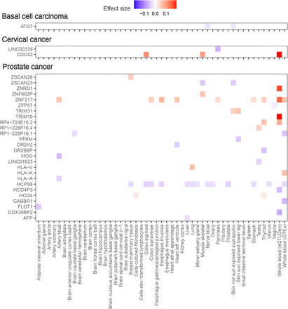
To infer whether SNPs from the novel genomic regions impact cancer risk through altering DNA methylation (DNAm) or gene expression levels, we performed Mendelian randomisation (MR) analyses (see Methods). First, we applied single-instrument two-sample summary Mendelian randomisation (SMR) analysis together with heterogeneity in dependent instruments (HEIDI) testing [29] on tissue-specific gene expression data from GTEx (v8) (N = 65-573, European ancestry, [30]) and whole blood-derived eQTLs from eQTLGen (N =31,684, [31]). We could map novel regions to 57 tissue-specific mechanisms involving 29 genes (Figure S5, Supplementary data). For example, CDC42 expression in muscle skeletal tissue ( , p = 5.2 · 10−6), colon sigmoid tissue (
 , p = 1.0 · 10−5), and whole blood (
 , p = 1.1 · 10−11) showed a risk-increasing effect on cervical cancer development (Supplementary figure S5). Second, we analysed mQTL data from the GoDMC consortium (N =32,851) [32] using SMR with HEIDI testing (see Methods). The analyses provided evidence for 225 pleiotropic associations between DNAm probes and BCC, cervical and prostate cancers in the 16 novel regions (Bonferroni-correction at p < 0.05/2380, HEIDI filtering at p > 0.05, Supplementary data). Among these 225 associations, we found that 44 probes overlap with probes linked to 23 other cancers from the Pancan-meQTL database [24]; and 3 of these 44 probes were differentially methylated by means of the same mQTLs (Figure 1c). This colocalisation analysis shows that our novel discoveries, in part, overlap with regions previously found to be methylated in tumour cells, implying that previous methylation differences in tumour cells are driven by germline variation.
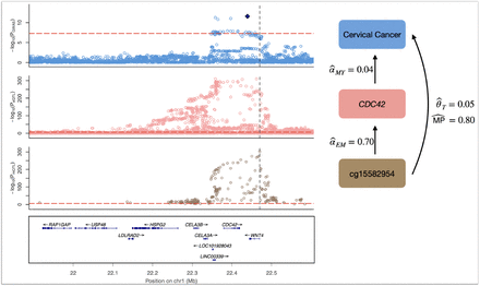
We further extended the MR analysis to multivariable MR (MVMR) to jointly estimate whether cancer SNP associations could be mapped to regulatory mechanisms of the scheme DNAm → gene expression → cancer in a genome-wide screen (see Methods). To maximise statistical power, we used mQTL and eQTL derived from whole blood as provided by the GoDMC and eQTLGen consortia, respectively, and conducted MVMR analyses to quantify mediation between DNAm (exposure E) and cancer traits (outcome Y) through gene expression (mediator M). Among the novel regions, the risk for cervical cancer was found to be increased by increased CDC42 expression (M → Y effect  , p = 2.4 · 10−8) through methylation at the cg15582954 probe (chr1:22’470’343; E → Y total effect
  , p = 3 8 · 10−8; Supplementary figure S4) corroborating findings from the tissue-specific MR analyses. CDC42 has been shown to be overexpressed in a number of human cancers and found to be a promising drug target in preclinical studies [33]. The GWAS signal physically locates closer to WNT4 than CDC42 (Table 1), however, a putative causal role of WNT4 in addition to CDC42 could not be assessed due to a lack of corresponding eQTLs for this gene [31]. Additional DNAm-to-gene expression mechanisms for previously identified cancer regions are listed in Table 2 and include mediation through genes well known to be implicated in cancer such as PDK1 [34], LYNX1 [35] and NEK10 [36].
Estimates from multivariable Mendelian randomisation (MR, see Methods), which was used to quantify mediation through gene expression for significant DNAm-to-cancer MR total effects. This provides a list of genes through which germline variation alters altering methylation, which changes gene expression, and in turn influences cancer risk. The mediation proportion quantifies the proportion of mediated causal effect (DNAm → Gene → cancer) relative to the total effect (DNAm → cancer).
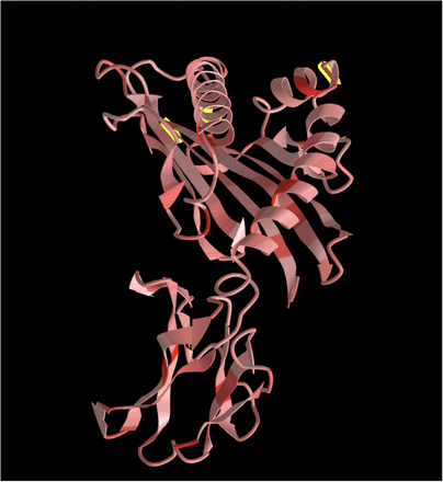
Finally, we assessed shared molecular functions of these genes and nearest to the novel SNPs genes using FUMA GENE2FUNC [37] software and the KEGG database [38]. The methylation and expression MR analyses identified cancer-specific gene targets whose regulation was changed by SNPs from the novel genomic regions, with a full list of potential novel genes given in Supplementary table S4. The genes were enriched in pathways of linoleic acid metabolism, interferon-gamma signalling, human papillomavirus infection, proteoglycans in cancer, axon guidance and viral carcinogenesis. Besides these pathways, the genes prioritised by FUMA using positional, eQTL, and chromatin mapping showed enrichment in lipids, steroids, and cholesterol metabolism, pathways in cancer, Kaposi sarcoma-associated herpesvirus infection, alcoholic liver disease, chemokine and Rap1 signalling pathway, microRNAs in cancer, as well as interferon signalling and antigen presentations pathways related to MHC-complex. Notable genes driving these discoveries are KRAS, CDC42, and WNT4, part of pan-cancer pathways, and the FADS complex associated with metabolism. Moreover, we closer examined the effects of exonic mutations from the novel genomic loci: 7 SNPs map to exons representing 5 nonsynonymous (HLA-A (3), TFAP4, ZBED2 genes) and 2 synonymous (ATG7, SLC6A18 genes) substitutions. We mapped 3 of these nonsynonymous mutations to the 3D protein structure of the HLA-A complex, where all substitutions fall into alpha-3 domains that form the binding groove that holds a peptide for presentation to CD8+ T-cells (Supplementary figure S11). In summary, our novel findings confirm previous pathways, highlight tumour associated methylation patterns that likely stem from germline variation, and provide additional potential mechanisms through which germline variation can affect cancer risk.
Genetic architecture of 11 cancers
We then aimed at estimating the genetic heritability of the 11 cancers using LD score regression on the marginal associations [39]. When correcting for the discrete nature of the trait (see Methods), the liability-scale heritability estimates were similar or higher and more precise than array-based assays except for non-Hodgkin’s lymphoma (Table 3), indicating that heritable genetic variation is a leading risk factor for underlying risk of cancer. The pattern holds even if we use an approach tailored for estimating liability scale heritability for rare traits [40] resulting in slightly more conservative estimates (Table S6). Interestingly, we find that the GMRM-BayesW analysis leads to nominally higher heritability estimates for many cancers than the GMRM-BayesRR-RC estimates, suggesting a better description of genetic architecture when including the timing information in the analysis. The joint Bayesian models for occurrence also enable SNP heritability estimation and comparative inference across cancers of the underlying distribution of genetic effects. The liability scale heritability estimates from the joint Bayesian model are similar to the LD score regression analysis estimates for more prevalent cancers. However, more remarkable differences between the estimates and wider credibility intervals occur for the less prevalent cancers, supporting suggestions [40] that rare traits require extra care as they could be subject to ascertainment bias, sampling bias, and their effective sample size is low. We further used cross-trait LD score regression on the BayesW or BayesRR-RC adjusted marginal associations to estimate the genetic correlation between the traits (see Methods). There is a sizable genetic correlation between melanoma and basal cell carcinoma (BayesW estimate 0.51, 95%CI 0.34-0.68), and we replicate [7] a previous result of negative genetic correlation between endometrial and testicular cancer (BayesW estimate -0.38, 95%CI -0.68 - -0.07) (Supplementary table S5). Interestingly, BayesW-based genetic correlations have a narrower confidence interval than BayesRR-RC based genetic correlation estimates for each significant cancer trait pair.
Estimates with 95% CI from LD Score regression, using mixed linear association model estimates adjusting for age-at-onset (GMRM-BayesW) or not (GMRM-BayesRR-RC), as compared with previous array or family based estimates. a - estimate from Rashkin et al. [7]; b - estimate from Mucci et al. [71]; c - estimate from Kilgour et al. [72]; d - estimates from Czene et al. [73].
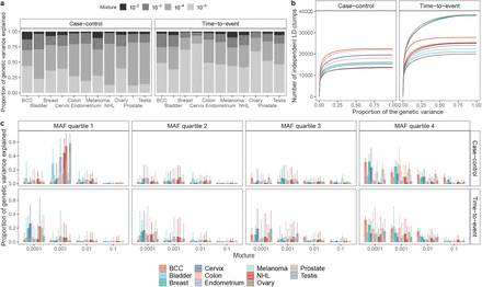
We find that all traits are highly polygenic, with most of the  attributed to SNPs that contribute an average of 0.1% and 0.01% of the group genetic variance for BayesRR-RC and BayesW models, respectively (Figure 2a). We find some differences across cancers, notably melanoma (10%), basal cell carcinoma (13%), breast (8.0%), cervical (5.1%), and prostate (5.4%) cancers; and for age-at-diagnosis of non-Hodgkin’s lymphoma (7.0%), bladder (6.0%) and ovarian (5.3%) cancers where at least 5% of the
  can be attributable to a small number of large effects (mixture 10−2) (Figure 2a). In general, the analysis of time-to-event phenotypes results in more of the genetic variance assigned to the smallest mixture component (Figure 2a). The result is in line with the number of LD-independent regions required to explain a proportion of the SNP heritability, where time-to-event analysis results in a more polygenic architecture compared to the case-control analysis (Figure 2b). Each curve reaches a plateau with 80-90% of the genetic variance attributable to a small number of genomic regions, and the remaining 10-20% attributable to 10,000 to 20,000 LD-independent regions. The number of remaining regions required to capture all of the association signals varies greatly across cancers, from 13,600 for ovarian and testicular cancer to 22,500 for basal cell carcinoma (Figure 2b). Additionally, we find that the 11 cancers differ in how rare and common variants contribute to the SNP heritability (Figure 2c). We further observe that genetic variance often positively correlates with variants’ MAF structure. For example, the largest proportion of genetic variance is consistently attributable to common variants in the fourth MAF quartile for both time-to-event (TTE) or case-control (CC) models on basal cell carcinoma (TTE 66%, CC 68%), melanoma (TTE 32%, CC 36%), breast (TTE 44%, CC 70%), colon (TTE 43%, CC 36%), and prostate cancers (TTE 40%, CC 57%) (Figure 2c). In contrast, testicular cancer, non-Hodgkin’s lymphoma and ovarian cancer have 61%, 54%, 63% of the genetic variance explained by the rarest effects in the first MAF quartile according to the case-control model. Thus, our MAF-LD Stratified
  estimation approach suggests: (i) strong differences in the underlying genetic architecture across these 11 cancers, (ii) that only a limited number of genomic regions are required to capture most of the risk for all cancers, and (iii) that mapping further associations will be extremely difficult as a small amount of variance is attributable to a large number of independent regions of the DNA.
(a) Mean proportion of genetic variance explained by each of the mixtures components using either case-control or age-at-onset phenotype. We find evidence that age-at-onset is highly polygenic with most of the genetic variance attributable to SNPs contributed by markers in the 10−4 mixture group, while the majority of the case-control phenotype genetic variance is explained by the markers from the 10−3 mixture group. (b) Number of LD-independent regions (see Methods) needed to explain total genetic variance. The contributions of LD-independent regions were sorted ascendingly such that the smallest contributing regions were added first. (c) Median proportion of genetic variance explained by each mixture class and MAF quartile combination, with 95% CI. For both case-control and age-at-onset models, most of the genetic variance is attributable to the small effect common variants (MAF quartile 4), however rare variants from the first MAF quartile contribute significantly to the variance for bladder, endometrial, ovarian, testicular cancers, non-Hodgkin’s lymphoma for the BayesR model. BCC indicates basal cell carcinoma.
Genomic prediction of 11 cancers
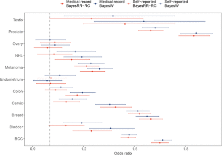
Next, we used BayesW SNP marker estimates to predict the occurrence of cancer in 195,432 individuals within the Estonian Biobank data (Figure 3, see Methods). We compared our results to those obtained by a baseline BayesRR-RC model, and also to SNP marker effect estimates obtained by Rashkin et al. [7] which combine the UK Biobank (408,786 European ancestry individuals; 48,961 cancer cases) and the Kaiser Permanente Genetic Epidemiology Research on Adult Health and Aging cohorts (66,526 European ancestry individuals; 16,001 cancer cases) to obtain a larger sample size. Additionally, we also compare our prediction estimates to the results obtained by Kachuri et al. [41] where they combined GWAS summary statistics across many cancer studies to achieve a much larger sample size. We provide a comparison of applying Bayesian models on either self-reported or medical record data (see Methods), showing that medical record data models outperform models using self-reported data. Thus, we resorted to using only medical record data (Figure S10), which illustrates the importance of high data quality and accurate measurement to facilitate phenotype linking across studies.
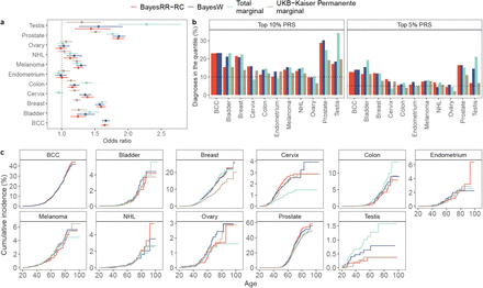
(a) Odds ratio for diagnosis of a tumour given one standard deviation increase in PRS, with 95% confidence intervals. (b) Percent of individuals diagnosed with cancer before age 50 having a top 10% or top 5% highest PRS; (c) cumulative incidence curves adjusted for competing risk for individuals with the top 5% highest PRS. The number of Estonian Biobank individuals used in the validation was N =195,432. BayesRR-RC and BayesW estimates were obtained by running the corresponding models on UK Biobank using either case-control or age-at-onset data. Total marginal estimates were obtained by using the marginal estimates that were concatenated from different GWA studies by Kachuri et al [41]. UKB-Kaiser Permanente estimates were obtained from the meta-analysis that combined analyes of UK Biobank and Kaiser Permanente cohorts [7]. We see that although BayesW and BayesRR-RC have the smallest sample sizes along with the smallest numbers of cases, the predictors uniformly perform better than a marginal analysis conducted on a slightly larger data set (UKB-Kaiser Permanente), and with a few exceptions it achieves similar or better predictive accuracy compared to the total marginal estimates that use effectively up to 10 times more tumour cases than BayesW and BayesRR-RC analyses. For all cancers except breast, cervical, endometrial and ovarian cancer, BayesW predictor gives a nominally higher odds ratios compared to BayesRR-RC predictor.
We find that Bayesian models for individual-level data, especially those utilising age-at-onset information, yield substantially improved genomic prediction for cancer occurrence, and the benefit is amplified as case count increases. Except for a few cancers for which none of the models gives significantly useful predictors, we find that conducting the analysis using an age-at-onset phenotype (BayesW) yields a nominally higher odds ratio (of having one standard deviation higher PRS) than a case-control phenotype (BayesRR-RC) for basal cell carcinoma (BayesW: 1.66, BayesRR-RC: 1.65), bladder cancer (BayesW: 1.36, BayesRR-RC: 1.24), colon cancer (BayesW: 1.19, BayesRR-RC: 1.16), melanoma (BayesW: 1.29, BayesRR-RC: 1.25), non-Hodgkin’s lymphoma (BayesW: 1.19, BayesRR-RC: 1.13), prostate cancer (BayesW: 1.86, BayesRR-RC: 1.85), and testicular cancer (BayesW: 1.55, BayesRR-RC: 1.44) (Figure 3a). A similar trend can be observed when using C-statistic or hazards ratio for comparison (Supplementary figure S9, see Methods). At least one of the Bayesian methods consistently outperforms previous analyses with a larger sample size that combine the biobank cohorts of the UK Biobank and Kaiser Permanente studies (UKB-KP) (see Methods). More notably, UKB-KP score has at least nominally smaller odds ratios (of standard deviation PRS difference) for testicular cancer (UKB-KP: 1.30), prostate cancer (UKB-KP: 1.51), breast cancer (UKB-KP: 1.23) and non-Hodgkin’s lymphoma (BayesW: 1.19, BayesR: 1.12, UKB-KP: 1.04). For the latter case of non-Hodgkin’s lymphoma, the UKB-KP score did not yield a significantly predictive score. The PRSs suggested by Kachuri et al. [41] combining multiple studies from a far more significant number of underlying cancer cases (Total marginal), yield mostly similar results to the BayesW and BayesRR-RC predictors using only UK Biobank data (Figure 3, Supplementary figure S9). For example, for breast cancer, where the previous study had 119,000 total cancer cases [9] as compared to our 17,000 cases (Supplementary table S1), we achieved similar odds ratios for standard deviation PRS change (BayesRR-RC: 1.59, Total marginal: 1.61). Bayesian scores outperform Total marginal PRS for prostate cancer (Total marginal: 1.77) and cervical cancer (Total marginal: 0.96), and Bayesian scores offer a marginal improvement for melanoma (Total marginal: 1.23) and non-Hodgkin’s lymphoma (Total marginal: 1.13). Testicular cancer stands out as both Bayesian scores perform noticeably worse compared to the Total marginal estimate, but here, our analysis resorted to only 886 cases whereas the previous risk score is combining more than 10,000 cases [13, 42] and thus the power in the UK Biobank in likely simply too low.
We observe that the highest 5% PRS quantile discriminates well for the disease occurrence (Figure 3c). Whereas the risk to develop prostate cancer by age 85 is estimated to be 11% (Supplementary table S7) among the top 5% highest PRS individuals, nearly 55% will develop prostate cancer according to the BayesRR-RC model. In comparison, UKB-KP PRS finds that 46% of the top 5% PRS develop prostate cancer. The top 5% polygenic risk score yields a useful discrimination rule for most other cancers as well, notably for breast cancer for which 19% of the top 5% BayesW PRS gets diagnosed with by age 85 (12% in the population, Supplementary table S7) and basal cell carcinoma for which 39% of the top 5% BayesRR-RC PRS gets diagnosed by age 85 (31% in the population, Supplementary table S7). The share of individuals getting a cancer diagnosis before age 50 is disproportionately higher among individuals with top 5% or 10% of the PRS across many cancers and risk score types (Figure 3b). For example, 23% out of all basal cell carcinoma cases and 30% out of all prostate cancer cases have the top 10% highest genetic risk according to BayesW risk score suggesting that the BayesW risk score discriminates well the early onset of prostate cancer or basal cell carcinoma. Our results suggest that the top 5% highest Bayesian polygenic risk scores could serve as a rule to detect individuals who should not only receive earlier communication about their risks but it could also result in a cost-effective screening model for this subset of individuals.
Discussion
Our results demonstrate the advantages of using joint Bayesian modelling and age-at-onset phenotypes for genomic prediction and GWAS discovery, highlighting how these approaches can be used to improve utilisation of existing data. Biobanks are becoming increasingly common worldwide, size and numbers of biobanks are increasing and improved links to electronic health record data enable information to be obtained regarding the age-at-diagnosis. Thus, we expect that our approach of incorporating age-at-onset data in the analysis will become commonplace, improving case-control studies by using richer information about the disease process.
One of the fundamental problems of analysing cancer phenotypes in a case-control fashion is the uncertainty that the control group subjects might later be diagnosed with cancer. Many cancers often become more prevalent only at later ages (Figure 3c), and as biobanks primarily consist of young, healthy individuals, it could distort the inference. That issue can be mitigated, for example, by introducing age thresholds to eliminate younger individuals who have been at risk only for a limited amount of time, or by age-matching individuals. However, this will always be somewhat arbitrary, it would reduce the sample size, and there is no guarantee that older individuals would not develop cancer in their later life. In contrast, time-to-event analysis treats these individuals as right censored, making no additional assumptions about the cancer occurrence in future. Therefore, time-to-event analysis suggests an alternative with a more sound conceptual background to yield more accurate inference. Interestingly, time-to-event adjustment tends to yield higher power than the case-control adjustment once the case count is high enough. Hence, time-to-event analyses could become more statistically powerful for future studies with potentially many added cases than their case-control counterparts at a high fixed case count.
Our PRS results remain limited as our work represents a re-analysis of a single biobank study, with the aim of demonstrating the methodological improvements that can be obtained. However, there is nothing preventing BayesW being run across different studies and posterior mean SNP effects being combined to improve the effectiveness of the PRS, providing predictors with the potential to stratify individuals for screening programs. For example, prostate cancer screening has been found to be only moderately useful for the general population with 17-40% [43, 44] reduction in cancer-specific deaths but as the mortality rate is low (in USA stage I-III 5-year survival rate >95%, stage IV 5-year survival rate 30% [45]) and as there are potential complications following the treatment, a general screening program has not been commonly implemented. Nevertheless, there are recommendations for stratified risk communication. For example, the American Cancer Society suggests that men with a first-degree relative with prostate cancer before age 65 should be informed about screening and its risks already at age 45, and men with multiple relatives with prostate cancer before 65 should be informed about screening even at age 40 [46]. Moreover, it has been found that even if screening is not cost-effective for men at average risk of prostate cancer, it is still cost-effective for men at very high risk (five times higher risk than the average) [44]. Our results suggest that the top 5% highest Bayesian polygenic risk scores could serve as a rule to detect those who should be screened and whose risk should be communicated.
There are important caveats to this study. Firstly, the discovery and training set of our study is limited to UK Biobank individuals with European ancestry whereas many other recent studies that have rather focused on merging and meta-analysing multiple data sets from various backgrounds. However, we replicate our findings on an independent data set and despite having a smaller discovery set we show that there are discoveries yet to be made on existing data set simply by using enhanced methodology for timing-related traits rather than occurrence-related traits. Secondly, the number of cancer cases is very low for some of our cancers such as testicular, ovarian or endometrial cancer leading to sub-optimal prediction accuracy, while cancers with higher case counts (prostate, breast) yielded good prediction accuracy. Hence, in future these analysis should be replicated with greater case counts for the cancers with smaller case counts. Thirdly, our current analysis combines both prevalent and incident cases to maximise the statistical power. However, it has been shown [7] that effect sizes are in general very similar even if we restrict the analysis only to incident cases. Future time-to-event analyses could also benefit from using information about left truncation by including entry date to the analysis, although the gain might be marginal as long as the phenotypic information is derived from the medical records and the onset happens later in life.
In summary, we have shown random effect models, especially those which utilise time-to-event data, maximise the use of existing data, for  estimation, genomic prediction and GWAS discovery of 11 common cancers.
Methods
UK Biobank Data
We restricted our discovery analysis in the UK Biobank to a sample of European-ancestry individuals. To infer ancestry, we used both self-reported ethnic background (UK Biobank field 21000-0) selecting coding 1 and genetic ethnicity (UK Biobank field 22006-0) selecting coding 1. We also took the 488,377 genotyped participants and projected them onto the first two genotypic principal components (PC) calculated from 2,504 individuals of the 1,000 Genomes project with known ancestries. Using the obtained PC loadings, we then assigned each participant to the closest population in the 1000 Genomes data: European, African, East-Asian, South-Asian or Admixed, selecting individuals with PC1 projection < absolute value 4 and PC 2 projection < absolute value 3. Samples were also excluded if in the UK Biobank quality control procedures they (i) were identified as extreme heterozygosity or missing genotype outliers; (ii) had a genetically inferred gender that did not match the self-reported gender; (iii) were identified to have putative sex chromosome aneuploidy; (iv) were excluded from kinship inference; (v) had withdrawn their consent for their data to be used. We used genotype probabilities from version 3 of the imputed autosomal genotype data provided by the UK Biobank to hard-call the genotypes for variants with an imputation quality score above 0.3. The hard-call-threshold was 0.1, setting the genotypes with probability ≤ 0.9 as missing. From the good quality markers (with missingness less than 5% and p-value for Hardy-Weinberg test larger than 10−6, as determined in the set of unrelated Europeans) we selected those with minor allele frequency (MAF) > 0.0002 and rs identifier, in the set of European-ancestry participants, providing a data set 9,144,511 SNPs. From this we took the overlap with the Estonian Biobank data described below to give a final set of 8,430,446 markers. This provides a set of high quality SNP markers present across both discovery and prediction data sets. For computational convenience when conducting the joint Bayesian analysis we created an additional subset of markers by removing markers in very high LD, through the selection of the highest MAF marker from any set of markers with LD R2 ≥ 0.8 within a 1Mb window. These filters resulted in a data set with 458,747 individuals and 2,174,071 markers.
We used the recorded measures of individuals to generate the phenotypic data sets for 11 most common types of cancer: bladder, breast, cervix, colon, endometrium, ovary, prostate, testis, basal cell carcinoma, melanoma, and non-Hodgkin’s lymphoma. Then, we created time-to-event phenotypes using either self-reported data or the linked electronic medical records data. For the medical record data, we used UK Biobank field 40008 to get the earliest age at each cancer diagnosis together with fields 40006 and 40013 to indicate the ICD10 or ICD9 cancer type (Table S2). Individuals without an entry on those fields were considered censored and their time was set to their last known age alive (exact birth date imputed to day 15 of a month as only month and year are known) without a cancer diagnosis. Each individual i was therefore assigned a censoring indicator Ci that was defined Ci = 1 if the person had the event before the end of the follow-up period and Ci = 0 otherwise. For self-reported time-to-event phenotypes, we created a pair of last known time (averaged between assessments) without an event and censoring indicator Ci. Similarly to the medical record phenotypes, if the event had not happened, then the last time without having the event was defined as the last date of assessment centre or date of death visit minus date of birth. For creating the self-reported phenotypes, we used UK Biobank field 20001 for the presence or absence of certain cancer type and UK Biobank field 20007 for interpolated ages of individuals when the disease was first diagnosed; we excluded from the self-reported phenotype analysis individuals who said that they had cancer, but there was no record of the diagnosis age. In an attempt to further increase power and to account for potential missingness, for each individual who had self-reported data about cancer timing but no medical record data, we used used the self-reported age-at-diagnosis instead of treating the individual as censored. However, this approach only yielded marginal improvements compared to using purely medical record information (Supplementary figure S10). Finally, the case-control-phenotypes corresponding to the time-to-event phenotypes were defined as the censoring indicators Ci.
The analyses were adjusted for the following covariates: sex for sex-unspecific cancers, age in case-control analyses, UK Biobank recruitment center, home location, genotype batch and 20 first principal components (UK Biobank field 22009) to account for the population stratification in a standard way. For the analyses that used age-at-diagnosis as phenotypes we did not include any covariates of age or year of birth because these are directly associated to our phenotypes.
Estonian Biobank Data
For the Estonian Biobank data, 195,432 individuals were genotyped on Illumina Global Screening (GSA) arrays and we imputed the data set to an Estonian reference, created from the whole genome sequence data of 2,244 participants [47]. From 11,130,313 markers with imputation quality score > 0.3, we selected SNPs that overlapped with those selected in the UK Biobank, resulting in a set of 8,430,446 variants out of which 2,174,071 variants were used in the prediction analysis. The 60 previously unreported variants that were found significant in the marginal association analysis of UK Biobank (Table S3) were used in a replication analysis using the same Estonian Biobank individuals.
We created the phenotypes for the Estonian Biobank individuals using the respective medical record information. The occurrence of each of the cancers was defined by using the respective ICD10 codes exactly as it was defined for the UK Biobank medical record phenotypes (Supplementary table S2) by first defining the last known time person did not have a respective diagnosis. Individuals with a respective cancer diagnosis received a censoring indicator Ci = 1 and 0 otherwise that then defined the case-control phenotypes adjusted for covariates such as sex for sex-unspecific cancers and age.
Analysis with joint Bayesian models
We estimated the hyperparameters such as genetic variance and prior inclusion probability by grouping markers into MAF-LD bins as recent theory suggests this yields improved estimation [48–50]. We ran the BayesW model on the UK Biobank data with 8 MAF-LD groups that were defined as first splitting markers by MAF quartiles and then splitting each of those MAF quartiles into two LD score blocks (MAF quartiles are 0.007, 0.020, 0.102; median LD score in each quartile are 2.32, 3.33, 5.69, 9.25, from the lowest MAF quartile respectively). We decided not to split these groups further as the potentially low statistical power of cancer-related phenotypes could lead to many groups with zero genetic variance. Both BayesW and BayesRR-RC models were executed with mixture components (0.0001, 0.001, 0.01, 0.1) for each of the groups, reflecting that the markers allocated into those mixtures explain the magnitude of 0.01%, 0.1%, 1% or 10% of the group-specific genetic variance. We ran the BayesW model using the timing of cancers as the phenotype while treating individuals without cancer as censored, and we ran the BayesRR-RC type model using the occurrence of cancer as the phenotype. In the BayesW analyses we took the covariates into account by estimating the effects of the covariates within the BayesW model while in the BayesRR-RC we regressed out the covariates from the phenotype prior to the analysis.
We specified the hyperparameters for the models such that they would be weakly informative. For BayesW model, the choice of hyperparameters and quadrature points was exactly the same as in [20]; for BayesRR-RC model the choice was exactly the same in [50]. We ran the chains for each of the cancer types twice for 6000 iterations, discarding the first 2000 iterations as a burn-in and using a thinning step of 5, leaving us with a final of 1600 samples of the posterior distribution. As estimation is done in parallel, the run time will depend on the degree of parallelisation. For example, for basal cell carcinoma we used 11 nodes and 12 tasks per node (total 132 tasks) for BayesW and 7 nodes and 12 tasks per node (total 84 tasks) for BayesRR-RC. This resulted in a total run time of 67.5 hours (40.5s per iteration) for BayesW and 79.7 hours (47.8s per iteration) for BayesRR-RC. Although BayesW was faster in the absolute time, adjusted for the number of tasks in the example, BayesW requires 33% more time per iteration than BayesRR-RC. Other choices for parallelisation (for example synchronisation rate) were set the same as described in [20].
Association testing with adjusted marginal models
For association testing, we used binary case-control phenotypes of cancer occurrences as a baseline. From those binary phenotypes we regressed out sex, (if applicable for the cancer), age, UK Biobank assessment centre, coordinates of birth place, genotype chip, and the leading 20 PCs of the SNP data. In addition, when testing each chromosome we regressed out from the phenotype the genetic effects of all the other chromosomes and the genetic effects were calculated using either the BayesRR-RC or BayesW models. That is, for every chromosome k, the phenotype was defined as
 where
where  matrix of SNPs in the lth chromosome,
  is the vector of average effect sizes from joint Bayesian analysis in chromosome l,
  is the binary phenotype that has been adjusted for covariates. Then, at each chromosome k we fitted the linear model for every marker j
 where
where  is the vector of jth marker values, βj is the jth SNP effect that we are estimating,
  is the error term with an error variance
  . Therefore, we estimated the effect size and standard error for each of the SNPs and we tested the significance using two-sided Wald test with a null hypothesis of βj = 0. For comparison, we also estimated the conventional unadjusted models where we did not adjust the phenotype for the genetic effects of other chromosomes, that is
 We used the full overlap of UK Biobank and Estonian Biobank markers giving us a total of 8,433,421 markers to be analysed. We used p-value threshold of 5 · 10−8 to determine the significance of each marker.
We applied the following steps on the association results to filter out independent and potentially previously undiscovered markers. Firstly, we LD clumped the results such that the index SNPs would have a p-value below 5 · 10−8 and SNPs could be added to a clump if they were 1Mb from the index SNP, they were correlated with r2 > 0.05 and they were nominally significant (P < 0.05). Next, we used COJO method [51] from GCTA software [52] to find clumps with independent signals by conducting stepwise selection of index SNPs in 1Mb window and we considered SNPs independent if they had a p-value below 5 · 10−8 in the joint model. To determine novelty, we first removed all markers that were significantly associated in the unadjusted model (eq. 3). We then removed all the markers that had a correlation of r2 > 0.1 with a marker that had been previously found associated with a cancer of interest using GWAS Catalog (published until July 2021) and LDtrait tool with the British in England and Scotland population. We then again used COJO to condition the remaining markers on the previously identified associations for each cancer of interest and SNPs that did not fall below 5 · 10−8 in the joint model were eliminated. For the remaining SNPs we conducted an additional literature review using Phenoscanner database [53, 54] to find any previous associations with variants of interest or variants in LD. The remaining candidates of novel associations were concatenated across BayesW or BayesRR-RC adjusted analyses and then included in the replication analysis using the largest available studies conducted for each specific cancer type. We were able to use studies with around 80,000 prostate cancer cases [11], 120,000 breast cancer cases [9]. We also checked findings for replication in the Estonian Biobank. Replication was defined as Benjamini-Hochberg corrected p-value being lower than 0.05 and the direction of the effect size same in both the original analysis and the replication analysis.
Liability scale heritability and genetic correlation
We used the summary statistics from the marginal association analysis in LD score regression [39] to calculate the observed scale heritability. We used the LD scores from the 1000 Genomes European data https://alkesgroup.broadinstitute.org/LDSCORE/ and the summary statistics were taken from either BayesW-adjusted or BayesRR-RC-adjusted association analysis. The conversion of the heritability to the liability scale was done using the formula by Lee et al. [55] (Table 3) and using the risks from SEER 2016-2018 (Table S7) [56] using the risks of having cancer diagnoses between ages 0 to 85 for non-hispanic white people providing similarity with the study population (European ancestry, UK Biobank, oldest person age 86). We further provide an alternative liability scale transformation [40] designed for rare traits. Using the alternative rare trait liability scale transformation we also present the heritability estimates from the joint Bayesian case-control model (Table S6). In addition, we used cross-trait LD score regression [57] to calculate the genetic correlations using results from BayesW or BayesRR-RC adjusted analyses, again using LD scores from the 1000 Genomes European data.
Discovery follow-up analyses
We conducted a number of follow-up analyses using the mixed-linear age-at-onset adjusted association model (GMRM-BayesW) and the baseline mixed-linear age-at-onset adjusted association model summary statistics.
Functional annotation analysis
We used FUMA (Functional Mapping and Annotation) [37] platform to functionally characterise novel replicated variants and prioritise genes. We defined a threshold for independent significant novel SNPs and corresponding novel genetic regions as LD r2 = 0.6 on the reference panel UKB/release2b. When performing gene mapping, we used 10kb maximum distance for positional mapping, all available tissue types and maximum p-value threshold of 5 · 10−8 for eQTL mapping, and builtin chromatin interaction data with 1 · 10−6 FDR threshold for chromatin interaction mapping.
We annotated SNPs by function and identified nearest genes using ANNOVAR [58], performing a two-sided Fisher’s exact test for quantification of functional classes enrichment. We obtained RegulomeDB categorical score [23], eQTL information, 15-core chromatin state [25], and CADD deleteriousness score [28] from SNP2GENE analysis of FUMA. We considered markers as deleterious if their CADD score exceeded the 12.37 threshold suggested by Kircher et al. (2014) [28] and chromatin state as open/active for SNPs with 15-core chromatin score ≤7 predicted by ChromHMM [25] based on 5 chromatin marks for 127 epigenomes. We annotated the SNPs with DeepSEA, a deep learning-based model that predicts chromatin effects of sequence variants and priorities regulatory variants, and we report here the functional significance score [26], maximum mean log e-value (MLE), and disease impact score (DIS) [27]. We calculated all of the mentioned parameters for each significant independent novel SNP as well as minimum/maximum/common values within the novel genetic regions.
We visualised the location of the exonic SNPs on a 3D protein structure by identifying amino acid substitutions in the gnomAD database [59], aligning proteins using Protein BLAST [60], and visualising with iCn3D Structure Viewer [61].
Mendelian randomisation analysis
We applied two-sample summary-data-based Mendelian Randomisation (SMR) and heterogeneity in dependent instruments (HEIDI) method [29] to assess genetic colocalisation between the 16 novel regions identified by our mixed-linear model BayesW analyses and DNA methylation (DNAm) as well as tissue-specific gene expression. DNAm levels were instrumented by mQTL data derived from whole blood provided by the GoDMC consortium (N =32,851, [32]). Tissue-specific eQTL data came from the GTEx consortium (v8) for 49 tissue types (N = 65-573, European ancestry, [30]). Additionally, we used whole blood-derived eQTLs from the eQTLGen consortium (N =31,684, [31]). We selected cis-m/eQTLs (< 1Mb of associated probe, p < 1 · 10−6) from the novel regions (if available in the investigated tissue) and conducted SMR-HEIDI tests using the top m/eQTL for each DNAm/gene probe, respectively. Given that most tissue-specific gene expression levels cannot be instrumented by multiple independent instrumental variables (IVs), the SMR-HEIDI approach was chosen over other MR methods that need multiple IVs to test for robust causal associations [62]. SMR outputs were also filtered based on a stringent HEIDI threshold of p > 0.05 [29]. Significance of gene-cancer SMR pleiotropic associations was defined at a Bonferroni-corrected threshold accounting for 1,825 (p < 2.7 · 10−5) tests summing across different tissues and instruments.
We further conducted multivariable MR (MVMR) to dissect significant DNAm-to-cancer causal effects (θT) into direct (θD) and indirect effects through transcript levels following the methodology outlined in [63]. While the previous SMR analysis was restricted to the 16 novel regions, the MVMR framework was applied on genome-wide GMRM-BayesW estimates across the 11 cancers. MVMR necessitates multiple IVs and we based the analysis on mQTLs and eQTLs from the GoDMC and eQTLGen consortium, respectively.
First, we conducted univariable inverse-variance weighting MR (MR-IVW) analyses for every exposure E DNAm probe with at least 5 near-independent instrumental variables (r2 < 0.05, p < 1 · 10−6, < 1 Mb from DNAm probe, ∼50,000 DNAm probes) accounting for correlated instruments [64] to obtain DNAm-to-trait total causal effect estimates (E → outcome Y effect  ). DNAm-trait pairs with an associated Bonferroni-corrected significant causal effect (pT < 0.05/50,000 = 1 · 10−6) were retained and distance-pruned (> 1 Mb) based on pT to be independent of each other.
Second, MVMR analyses were performed to estimate the direct effect  by including transcript mediators (M) and their associated genetic instruments (p < 1 · 10−6). Transcripts were required to be in cis (< 500kb away from the DNAm probe) and causally associated to the DNAm probe. This latter condition was verified by calculating univariable MR-IVW effects from the DNAm probe on the transcript to estimate a causal effect
  and associated p-value pEM (significance was defined at pEM < 0.01). Analogously to the total causal effect estimation, direct effects
  were then calculated in an MVMR regression accounting for correlation among IVs [65]. The mediation proportion
  was then estimated as
  . Causal effect estimates from the transcript mediator on the outcome trait
  were obtained from univariable MR-IVW analyses.
To ascertain that MVMR estimates did not suffer from heterogeneity, which could point towards horizontal pleiotropy, we computed heterogeneity tests based on Cochran’s Q-statistic [66]. Homogeneity within the genetic instrument set was assured at pHET > 0.01.
We compared the significantly associated methylation probes from the novel regions with the Pancan-meQTL database [24] which provides meQTLs across 23 cancer types from The Cancer Genome Atlas. For this comparison, we used the probes identified by SMR (2,380 tests). The significance threshold was adjusted for the total number of tests (p < 0.05/2, 380 = 2.1 · 10−5).
For pathway analyses, we derived a list of genes whose differential expression was found to be associated with cancer risk based on the eQTL and mQTL MR analyses. For this, we combined results from the following analyses: single-instrument SMR on GTEx (v8) (1680 tests), eQTLGen (145 tests), and GoDMC (2380 tests) datasets and multi-instrument MR-IVW on eQTLGen (61 tests) and GoDMC (998 tests) datasets. The overall significance threshold on combined data was Bonferroni-corrected p < 0.05/5264 = 9.5 · 10−6. We used both the cis- and trans-meQTL datasets across 23 cancer types from the Pancan-meQTL database to identify methylation-related genes whose expression is affected by the SNPs from the novel regions. Finally, we extended the resulting list of genes by adding the nearest to the novel SNPs genes identified by ANNOVAR and protein coding genes from FUMA positional, eQTL, and chromatin interaction mapping. We then tested pathway enrichment with FUMA GENE2FUNC software [37] and KEGG Mapper [38].
Genomic prediction in the Estonian Biobank
The predictors based on BayesW or BayesRR-RC models into Estonian Biobank ĝ were obtained by multiplying the standardised genotype matrix with the average SNP effect across iterations
 where XEst is NEst × M matrix of standardised Estonian genotypes (each column is standardised using the mean and the standard deviation of the Estonian data),
  is the M I matrix containing the posterior distributions for M marker effect sizes across I iterations,
  is the average SNP effect. We calculated the average predictor from BayesW and BayesRR-RC models using for each cancer using 1600 iterations (see Analysis with joint Bayesian models). We compared our Bayesian risk scores with the ones provided by Kachuri et al. [41] (Total marginal) and the ones provided by Rashkin et al. [7] (UK Biobank - Kaiser Permanente). Total marginal estimate combines summary statistics from several studies (total 543 SNPS were used in total for 11 cancer scores, each score having an individual subset of SNPs) and they calculate the PRS using inverse variance weights that showed the best predictive performance. The PRS was thus calculated as the sum of standardised SNP dosage values in Estonian Biobank time inverse variance weighted SNP effects. Using the same idea of inverse variance weights, we combined 314 SNPs with weights from [7] to also get PRS for each Estonian Biobank individual.
We evaluated the performance of the 4 types of genetic predictors for each cancer phenotype by comparing them to the true phenotype case-control status using logistic regression and true phenotype timing using Cox proportional hazards (PH) model. The 4 predictors were compared using the top 5% PRS with the rest, the top 10% PRS with the rest and the comparing the effect of one standard deviation increase in PRS. From the logistic regression we calculated odds ratios for the top 5%, top 10% and scaled change effect. From the Cox PH model we calculated hazards ratios and Harrell’s C-statistics [67] for the top 5%, top 10% and scaled change effect. In addition to the predictor, gender (if applicable) and age-at-entry were included in the logistic regression and Cox PH model that was calculating the hazards ratio. Harrell’s C-statistic was calculated from the Cox PH model where the true phenotype was regressed only one the predictor. The results of odds ratios, hazards ratios and Harrell’s C-statistics are shown in Figure 3a and Supplementary figure S9. We further used the top 5% and top 10% PRS individuals to see what percentage of them develop a cancer (Figure 3b).
Across all the cancers and 4 predictive scores we calculated the respective cumulative incidence curves for the top 5% highest PRS individuals (Figure 3c) adjusting the analysis for the competing risks. The calculation was done using R package cmprsk [68, 69].
Author contributions
SEO and MRR conceived and designed the study. MRR, SEO, ESM designed the study with contributions from KL and MCS. SEO, ESM, KL, MCS and MRR contributed to the analysis. SEO, ESM, MCS and MRR wrote the paper. KL, ZK, RM provided study oversight, contributed data and ran computer code for the analysis. All authors approved the final manuscript prior to submission
Author competing interests
The authors declare no competing interests.
Data availability
This project uses UK Biobank data under project 35520. UK Biobank genotypic and phenotypic data is available through a formal request at (http://www.ukbiobank.ac.uk). The UK Biobank has ethics approval from the North West Multi-centre Research Ethics Committee (MREC). For access to be granted to the Estonian Biobank genotypic and corresponding phenotypic data, a preliminary application must be presented to the oversight committee, who must first approve the project, ethics permission must then be obtained from the Estonian Committee on Bioethics and Human Research, and finally a full project must be submitted and approved by the Estonian Biobank. This project was granted ethics approval by the Estonian Committee on Bioethics and Human Research (https://genomics.ut.ee/en/biobank.ee/data-access).
Code availability
The BayesW model was executed with the software Hydra, with full open source code available at https://github.com/medical-genomics-group/hydra [70]. Summary MR-HEIDI tests were conducted using the SMR software (version 1.03) [29]. The multivariable MR analyses were carried out with SMR-IVW extension software https://github.com/masadler/smrivw. plink version 1.9 is available at https://www.cog-genomics.org/plink/. R version 4.0.3 is available at https://www.r-project.org/.
Supplementary material
Supplementary tables
For each of the tumour types, the corresponding ICD10 and ICD9 codes are presented that were used to define cancer occurrence.
We observe that for the 59 previously unreported variants, the p-value in the unadjusted association analysis is borderline significant (5 · 10−8 < p < 10−4) and by using the BayesW or BayesRR-RC adjustments, we arrive at statistically significant test statistics.
We combined results from the following analyses: single-instrument SMR on GTEx (v8) (1680 tests), eQTLGen (145 tests), and GoDMC (2380 tests) datasets and multi-instrument MR-IVW on eQTLGen (61 tests) and GoDMC (998 tests) datasets. The overall significance threshold on combined data was Bonferroni-corrected p < 0.05/5264 = 9.5 · 10−6. The genes affected by differentiated methylation were taken from the Pancan-meQTL database. Finally, we extended the resulting list of genes by appending the nearest to the novel SNPs genes and protein coding genes from FUMA positional, eQTL, and chromatin interaction mapping.
We calculate the genetic correlations between cancers with cross-trait LD score regression [57] applying it on the results from BayesW or BayesRR-RC adjusted analyses. LD scores for the analysis were taken from the 1000 Genomes European data. Both BayesRR-RC and BayesW based significant genetic correlations agree on the magnitude of the estimates but BayesW based estimates result in narrower confidence interval than the BayesRR-RC based estimates.
We use the observed scale from LDSC estimates (summary statistics from BayesW-adjusted analysis) and the heritability estimates from the full Bayesian model (BayesRR-RC). Transformation of the observed scale heritabilities are done with a more conservative approach (Ojavee et al. [40]) better suited for rare diseases.
To ensure that the lifetime risk estimates were similar to the study population (European ancestry, UK Biobank, oldest individual age 86) we used the estimates from SEER of non-hispanic white of getting diagnosed between ages (0-85). The explorer is accessible from https://seer.cancer.gov/explorer/. The explorer had a joint estimate for colorectal cancer that we transformed to the risk of colon cancer using the proportion of colon cancer cases among colorectal cases (70.3%, https://www.cancer.org/cancer/colon-rectal-cancer/about/key-statistics.html, accessed 24.01.2022). For basal cell carcinoma we used lifetime risk estimate from Miller et al. [74].
Supplementary figures
We observe that in general BayesW or BayesRR-RC LOCO adjustments result in decreased p-values suggesting an increase in statistical power. Furthermore, for most traits, BayesW adjustment results in even lower p-values compared to the ones resulting from BayesRR-RC adjustment.
Among previously reported variants both case-control and age-at-onset adjustments most commonly discover same variants in our analysis. Time-to-event adjustment suggests to give more associations than case-control adjustment and that mostly for cancers with high case count (prostate cancer, breast cancer, basal cell carcinoma). The replication rate is slightly better for variants that had been discovered using time-to-event adjustment.
The discovery data set results are based on the UK Biobank analysis whereas replication for most traits was done in the Estonian Biobank with the exception of prostate and breast cancers for which we used previously published results combining larger sample sizes. Fisher’s exact test testing the independence of the signs of the replication/discovery z-scores resulted in a p = 0.0016 indicating that the z-scores coming from replication or discovery sets are dependent.
The first three rows display the genetic associations (-log10(p-values)) from top to bottom with cervical cancer (blue), CDC42 transcript levels (pink) and DNAm probe cg15582954 (brown), respectively. The solid diamond in the GWAS locus plot represents the top SNP in LD with the novel GWAS discovery. Red dashed horizontal lines indicate the significance thresholds of the respective SNP associations and the vertical black dashed line represents the DNAm probe position. The bottom row illustrates the positions and strand direction of the genes in the locus. On the right side, a schematic of the regulatory mechanism with calculated MR effects and mediation proportion (MP) is shown.
We conducted SMR-HEIDI tests using novel SNPs or the SNPs in LD with the novel SNPs as instruments. Plotted are the significant Bonferroni-corrected associations that survived HEIDI filtering.
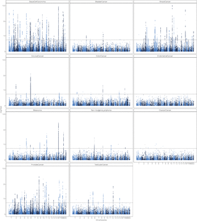
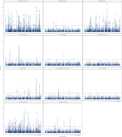
The significance of each SNP was tested using binary (case-control) phenotype indicating cancer occurrence that was adjusted only for covariates. Number of markers analysed was M =8,430,446, the number of individuals and cases for each specific cancer are shown in the Supplementary information. For each of the markers a two-sided Wald test was carried out with a null hypothesis of a marker having no effect on the adjusted phenotype. We present the − log10(p-value), the dotted line indicates a significance threshold of p = 5 · 10−8.
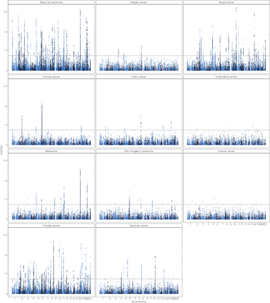
The significance of each SNP was tested using binary (case-control) phenotype indicating cancer occurrence that was adjusted for covariates and BayesW genetic predictor using the effects from all of the other chromosome (leave out one chromosome). Number of markers analysed was M =8,430,446, the number of individuals and cases for each specific cancer are shown in the Supplementary information. For each of the markers a two-sided Wald test was carried out with a null hypothesis of a marker having no effect on the adjusted phenotype. We present the − log10(p-value), the dotted line indicates a significance threshold of p = 5 · 10−8.
The significance of each SNP was tested using binary (case-control) phenotype indicating cancer occurrence that was adjusted for covariates and BayesRR-RC genetic predictor using the effects from all of the other chromosome (leave out one chromosome). Number of markers analysed was M =8,430,446, the number of individuals and cases for each specific cancer are shown in the Supplementary information. For each of the markers a two-sided Wald test was carried out with a null hypothesis of a marker having no effect on the adjusted phenotype. We present the − log10(p-value), the dotted line indicates a significance threshold of p = 5 · 10−8.
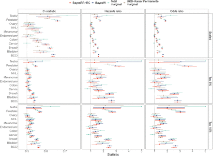
The statistics were calculated by finding the impact of one standard deviation increase in the PRS (Scaled), by finding the impact of belonging to top 5% quantile of the PRS or by finding the impact of belonging to the top 10% quantile of the PRS on the likelihood of having cancer. Harrel’s C-statistic was calculated from Cox proportional hazards model without covariates, odds ratio was calculated from a logistic model using sex and age-at-entry as covariates, hazards ratio was calculated from Cox proportional hazards model using sex and age-at-entry as covariates.
The polygenic risk scores that are using medical record data rather than self-reported data tend to be more predictive across all cancers. The odds ratios were calculated by finding the impact of one standard deviation increase in PRS in a logistic model using sex and age-at-entry as covariates.
Three nonsynonymous mutations in the HLA-A complex (p.Arg68Lys, p.V al91Met, p.Ala174V al) are marked with yellow colour: all substitutions fall into alpha-3 domains that form the binding groove that holds a peptide for presentation to CD8+ T-cells.
Acknowledgements
This project was funded by an SNSF Eccellenza Grant to MRR (PCEGP3-181181), and by core funding from the Institute of Science and Technology Austria and the University of Lausanne.
K.L. and R.M. were supported by the Estonian Research Council grant PRG687.
Estonian Biobank computations were performed in the High Performance Computing Centre, University of Tartu.
We would like to acknowledge the participants and investigators of UK Biobank and Estonian Biobank studies.


