Predicting COVID-19 outbreak using open mobility data for minimal disruption on the country’s economy

1. Background

At the end of 2019, humanity has been challenged with a new pandemic caused by the novel corona virus identified as SARS-COV-2, leading to a global pandemic causing the disease called COVID or COVID-19. The outbreak was first identified in late December 2019, in the Wuhan province in China, when health authorities identified cases of atypical pneumonia of unknown origin and evidence of person-to-person transmission via droplets or direct contact [1] [2]. People were affected in different ways, developing mild to severe illness. Among the common symptoms were identified: fever, chills, muscle pain, headache, sore throat, cough, and shortness of breath (difficulty of breathing). After being infected with the virus, it can take up to 14 days for people to develop symptoms [3] [4]. According to World Health Organization (WHO), by the end of January 2020, China had more than 11,800 confirmed COVID-19 cases, as well as more than 250 deaths [5]. In a few months, the virus outbreak spread to countries in Asia, Europe, and America. On February 15th, 2020, WHO confirmed more than 40,000 cases in 28 countries. On March 11th, 2020, it also declared the outbreak as the Sixth Public Health Emergency and a global pandemic [6]. In order to avoid the increase on infections and overwhelm the health services of each country, WHO made the following recommendations:

• avoid close contact with sick people or with symptoms of COVID-19,

• avoid attending massive events as well as family gatherings,

• washing hands with soap and water for more than 20 seconds,

• cover mouth and nose with the elbow or a tissue when coughs or sneezes among others [1] [7].

Such contingencies measures that lead to greatest impact worldwide is social distancing such as travel and mobility restrictions as well as population confinement in their homes [8] [9].

Several countries adopted social distancing measures, such as self-quarantine, workplace and mobility restrictions in the public space, and facilities closures. Some of them in a voluntary manner by the citizens (such as Latin American countries) and others through strict mobility and travel restrictions (such as Spain, the United States, Italy or South Korea). All of these policies have the goal to reduce mobility in the public space, hence, reducing the probability of contact between non-infected and infected people, leading to avoidance of new community-transmitted cases [10][11][12][13]. For some countries, having the ability to measure population mobility variations is a challenge that must be solved in order to have data that helps predicting the spread of the disease. During this outbreak, predictive models have become a key tool for health authorities in each country to assess the level of saturation that health services might have. To date, no model has been able to accurately predict the evolution of future cases, however, depending on the variables involved, the number of people who could become infected and die, can be predicted.

Some authors have proposed different forecasting models. For example, a modified SEIR (Susceptible − Exposed − Infectious – Recovered) model to predict the COVID-19 outbreak was proposed by Löpez and Rodö [14]. They incorporated the effects of varying proportions of containment and fit data to quarantined populations accounting for the spread of infection during the outbreak. The proposed model predicts the number of infected individuals (undiagnosed) considering the different levels of isolation of the population, to evaluate the effects of the reduction of contacts. The model provides results similar to those obtained with more complex models. Li et. al [15] used the Gaussian distribution theory to propose a new model of COVID-19 transmission. The simulation results show that the curve of the proposed model is quite similar to the curve calculated with official data from different countries such as China, South Korea, Italy, and Iran. The model considers the virus incubation period, basic reproduction number, and daily infection number. A statistical forecast using time series models with open-data of confirmed cases, deaths, and recoveries was proposed by Petropoulos and Makridakis [16]. Using univariate time series models, and assuming that the data is accurate and that past patterns will continue to apply, forecast curves are obtained that could be used for decision-making and implementing control measures. The results obtained with these models show that forecast graphs of the COVID-19 outbreak can be calculated, however, none of them considers information on the people’s mobility to assess the effectiveness of the social restriction policies implemented in each country.

On the other hand, Oliver et. al [17] describe how mobile phone data could be used to design social distancing policies and delay the spread of the outbreak. The authors identified reasons why not all countries are able to use this information for predicting future cases. During the COVID-19 outbreak, some countries do not provide access to accurate information which might help to determine the mobility of their population and evaluate the effectiveness of social distancing policies. After WHO declared a global pandemic, Google© [18] and Apple© [19] released public mobility data from their platforms to help COVID-19 outbreak spread. Both companies decided to provide data about the people’s mobility patterns around the world based on information from mapping and GPS applications. Such information can be useful for health authorities as a basis for decision-making considering the volume of people who uses private vehicles, walks, or uses public transportation. Mexican government used this information to monitor people’s mobility in the public space [20].

As contribution, the authors propose a method for forecasting the outbreak using Google© and Apple©’s mobility trend reports. The authors envisions that this article can contribute to health authorities for making timely decisions, preventing the spread of viruses while balancing the reduction of mobility with minimal disruption in people’s economies in future outbreaks.

2. Technical Framework

In any infectious disease, there are a number of parameters to consider when countries are trying to control the outbreak. The most known parameter is vaccination, which allows to basically reduce to a manageable number of cases, ideally to zero. In cases with novel infectious agents such as the novel SARS-CoV-2 virus, which causes the disease called COVID-19, no vaccination yet exits, making public health officials being challenged to manage cases under control. For such cases, another parameter shall be used, called R which refers to the effective reproduction number [21] and, basically describes the way of measuring an infectious disease’s capacity to spread. In this study, the R number will be limited to understand outbreak spread [22], the use of it on the method and what it means for the average number of people that one infected person will pass the virus to [23].

The R number shall not be considered as a fixed parameter. Instead, it shall be seen as a parameter that can be affected by a range of factors [24], including not just how infectious a disease is but how it develops over time, how a population behaves in terms of mobility, containment and immunity. Immunity might be as a result of infection or vaccination.

A particular version of R is called R₀ and is referred as the basic reproduction number, which is used when a new infection disease is discovered [22]. Another common use of R is called R_e or the effective reproduction. Ideally this number with vaccination is lower than 1.0 [25] [26].

In the case of SARS-CoV-2, R value varies from country to country, people’s behavior and population’s density: in urban areas, larger R₀ values would be expected versus rural areas otherwise.

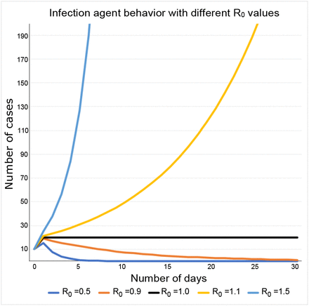
In order for any infectious disease such as the COVID-19 pandemic, is under control, R₀ should be below 1. If R₀ is equal to 1, then the outbreak is contained but never will disappear over the time. If R₀ is greater than 1, then public health systems might suffer depending how lethal the infection agent is. Figure 1 shows different behaviors to an infection agent with just 10 identified cases in day 0. Over the time, depending upon the R₀ value, cases might go down to zero (for R₀ values less than 1) or might go up (for R₀ values greater than 1). Hence the importance of controlling R₀ values to manage outbreak spreads.

• Download figure
• Open in new tab

Figure 1.

An infection agent such as SARS-COV-2 has a different behavior while reproduction number R₀ varies.

According to WHO, one of the main strategies to contain the SARS-CoV-2 outbreak is via social distancing [27], meaning that people should maintain a safe separation from another individual, but also avoiding crowded places mainly in the public space. National state governments might adopt different measures to maintain social distances, some of them aiming public will and some others using enforcement agencies such as the police or national guards. The most important aspect is to keep people away from crowded places such as schools, public locations, office buildings, shopping centers and manufacturing floors.

Most of the national governments should keep a balance between public health, domestic macroeconomics and society well-being in general. Given the current outbreak conditions where there is no other treatment but keeping social distance, it results extremely important to make a decision on when the reduction in mobility should be in place and how deep this reduction should be applied in the public life. In this paper the authors propose a method to anticipate the growth of SARS-COV-2 in urban areas using open mobility data coming from Apple© iOS and Google© Android mobile phones. In addition, lessons learned from successful countries controlling the pandemic are discussed.

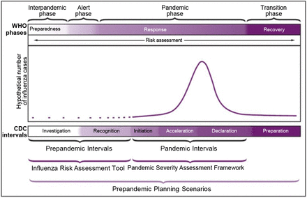
According to WHO there are four phases in a pandemic: Interpandemic phase, Alert phase, Pandemic phase and Transition phase, whereas the US Centers for Disease Control and Prevention, CDC, refers to 6 intervals: Investigation, Recognition, Initiation, Acceleration, Deceleration and Preparation. Figure 2 describes the pandemic curve of any infectious agent and both WHO and CDC phases or intervals. It is of our interest to understand the behavior of an outbreak in order to make the intervention measure more effective with the use of mobility data. Most of the current forecasting models [14][15][16] use the number of existing cases and make projections of future case growth using the expected outbreak scenario with and without interventions.

• Download figure
• Open in new tab

Figure 2.

Preparedness and response framework for novel influenza A virus pandemics, with CDC intervals and WHO phases [28].

According to the Community Mitigation Guidelines to Prevent Pandemic Influenza [29] there shall be a risk assessment to understand the deepness of measures such as closure of schools or workplaces as well as the reduction of people’s mobility in the public space.

Table 1 shows the initial assessment in terms of transmissibility and clinical severity. As seen on the table, R₀ greater than 1.8 means a moderate to high risk, as well as a case fatality rate greater than 10%. Hence the importance of predictive models that allow health officials to make decisions aiming to keepx R₀ at low values.

For a specific country or location, the future case growth can be expressed as a function of its population mobility parameter called m₀, and its basic reproduction number R₀.

Table 2 shows that different values of R₀ and the impact in future case growth with only 10 cases in day 1 and assuming R₀ is not affected. According to pandemic mitigation this action would be referred as a scenario with no intervention [31]. Equation 1 shows the case growth based on R₀:

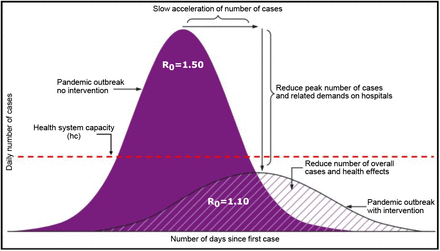
where: The importance of mobility parameter m₀ in pandemic mitigation for COVID-19 is key to make the cases below the health system capacity h_c shown in Figure 3. Herein, the main contribution of this method is on finding the proper mobility m₀ parameter via public mobility data such that cases never overpasses h_c. Ideally h_c value shall be below maximum capacity to avoid saturation of public health system or within a toleration threshold given that health capacity will not be overpassed.

• Download figure
• Open in new tab

Figure 3.

Adapted from: CDC. Interim pre-pandemic planning guidance: community strategy for pandemic influenza mitigation in the UnitedStates— early, targeted, layered use of nonpharmaceutical interventions and capping to Health System Capacity [31].

3. Model and Data sets

As explained in section 2, the main goal of this research is to find how mobility impacts in future case growth and, eventually, be able to use mobility parameter m₀ as the controlling factor to reduce SARS-COV-2 transmission, in a form of case future growth reduction, given that there is no current vaccination available.

In general terms, the case growth can be represented as a function of the number of cases in the period i as C_i and its basic reproduction number R₀ as described in Equation 1. If i = 1 then C₀ is the initial case of the pandemic. In our case, this is the first documented case and this will indicate the first day of the epidemic curve.

When R₀ is greater than 1 and there is no intervention [31], then the number of cases tends to grow exponentially until the outbreak reaches its natural peak.

Herein the importance of R₀ to be controlled with some mechanism of intervention. In this case, the use of m₀ is proposed and for that matter, the use of mobility data provided by mobile applications such as Google© and Apple© data.

In this study, R_t means the temporal reproduction number. Consequently R₀ can then be represented as a function of m₀ parameter to smoothen the exponential growth of daily cases. Equation 2 shows this expression: where: to make Equation 1 can be rewritten as: R₀ and m₀ parameters are calculated in subsequent sections.

4. Results

Based on the numbers for CMI and R_t shown in Table 4, the behavior of these parameters was analyzed over the 6 periods of 14-days (with the exception of Mexico and Brazil, which spans for 78 and 81 days respectively). A 14-day rolling average of both parameters was calculated in order to understand the trend, if any, and finally a Pearson’s correlation between these two data sets of parameters on a per country-basis was done, in order to identify how much mobility, would impact the reproduction number.

In a Pearson’s correlation r statistic [36], when one variable increases the other variable has a tendency to also increase. This is called a positive correlation. A negative correlation indicates when one variable increases the other variable has a tendency to decrease. Finally, there is no correlation when one variable increases, the other variable does not tend to either increase or decrease [37].

Cohen [38] and Evans [36] proposed empirical classifications of interpreting correlation strength by using Pearson r statistic. Cohen recommended that 0.10 to 0.30 be interpreted as a weak correlation, 0.30 to 0.50 as a moderate correlation and greater than 0.50 as a strong correlation. According to Evans’ classification, less than 0.20 is very weak, 0.20 to 0.39 is weak, 0.40 to 0.59 is moderate, 0.60 to 0.79 is strong and 0.80 or greater is a very strong correlation for the absolute value of r [39].

A statistically significant correlation does not necessarily mean that the strength of the correlation is strong. In order to determine whether the correlation between variables is significant, it is necessary to compare the p-value to a significance level. The p-value shows the probability that this strength may occur by chance [40]. A significance level, denoted as α or alpha, of 0.05 is generally acceptable. This means that the risk of concluding that a correlation exists when no correlation exists is 5%.

Based on this analysis, using Evans’ classification and p-value<0.05, countries were classified in three main sets:

• Countries with Pearson values greater of 0.60 or with a strong to very strong correlation.

• Countries with Pearson values between 0.40 to 0.59 or with moderate correlation.

• Countries with Pearson values less than 0.39 or with weak or very weak correlation.

All of them under the assumption that p-value has a high statistical significance with p-value<0.05. As described, correlation strength is not enough, but is necessary to determine the statistical significance. The results of these new calculations are also shown in Table 5.

As shown in table 5, countries might have a positive or negative correlation, low or high correlation strength, but the most important value to make an initial decision if the proposed model would work is the statistical significance p-value. If p >0.05, then the correlation has not statistical significance, meaning the correlation between data sets is not significant, so can’t lead to any decision.

From table 5 can be seen that Brazil and Mexico have a strong correlation, meaning that their mobility reduction and reproduction rates were strong correlated, whereas Italy and Spain have weak correlations. Impact of cases growth for Italy and Spain is expected and could be seen with the correspondent impact on health systems overloads. The particular case of United States where there is a negative correlation is a clear indication that case might be out of control due to mobility increase. For the cases of South Korea and UAE, the authors do not recommend using this method because there is no statistical significance between the CMI and Rt values.

5. Discussion

The main goal of the proposed method is to find m₀ that contributes to control number of cases, which is a function of R_t subject to the health capacity system h_c.

Maximum number of cases will determine the potential number of people requiring hospitalization services, hence controlling R_t via m₀ is fundamental.

The proposed method is described below:

1. Given initial number of cases, determine R_ti as described in Section 3. Authors suggest to have at least two full 14-day periods of confirmed cases in order to provide an approximation of R_t. Remember that for the purpose of the calculations R_t = R_e.

2. Obtain daily CIM as described in Section 3. For the purpose of this research, Apple© and Google© Mobility Data was used, but any mobility data can be used.

3. A valid Pearson correlation of CIM and R_t pairs should be obtained. Authors suggest to calculate a p-value, such that p-value < 0.05 provides a valid statistical significance for Pearson correlation. The stronger Pearson correlation and the p-value <0.05, the better the validation of CIM and Rt will be.

4. Obtain 7-day rolling averages of CIM and R_t. For example, if the data set has 30 days of cases, then, 23 7-day rolling averages can be obtained.

5. Using the last CIM and Rt rolling averages as the seed data, projections can be done, where m₀ value could be changed to make R_e<1.

From Section 4, future case growth depends on initial number of cases but also in two determining factors:

• Number of confirmed cases in the second 14-day period, ideally in less than 40 days.

• Daily Effective Reproduction Number for the same period.

For the purposes of the discussion, R_t (temporal reproduction number) is in fact the R_e number for the pandemic wave, meaning that the effective reproduction number will be considered as the actual daily case growth. The bigger R_e were in that second period, a greater mobility reduction would be needed to decelerate future case growth.

However, the biggest challenge found in most of the predictive models relies on the fact that confirmed cases are cumulative and some countries may change their method to identify cases depending upon the pandemic behavior. Counting cases and expecting changes on cases is not scalable nor practical to analyze.

Also, none of the models suggests ways to control the behavior of the pandemic, so this is the opportunity this model is intended to address.

In order to describe the model from a practical perspective, actual cases from one country were chosen and its data is shown in Table 6. Number of daily confirmed cases from “Our World in Data” journal database [32] were used to calculate daily R_e using Equation 4. Daily CIM was calculated as well for the same period of time using Google© [18] and Apple© [19] mobility data. Selected country had a Pearson correlation of 0.58, moderate according to Evan’s model [36] with p-value of 0.001 with α = 0.05, in a period of 30 days.

Using this data, 7-day rolling averages were calculated for R_t and CIM data of both parameters was used as seed for projections, also shown in Table 6. Variable parameter for projections is a value of m₀ given that resulting R_t is less or equal to 1, hence number of cases will tend to stall or decrease over time. For this country, three scenarios were projected using the proposed method:

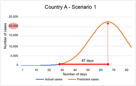
• Scenario 1: Light constant mobility reductions (CIM=-1) until reach R_e<1. Peak number of cases is about 22,400 cases with a total reduction of mobility of -81.5% to reach R_t=0.99 and keep going down. The disadvantage of this approach is a hard reduction in mobility of more than 80% for more than 60 days. This scenario is inviable for low-income economies and small and medium business companies. Figure 4 shows total number of cases and behavior over the time.

  

  • Download figure
  • Open in new tab

  Figure 4.

  Country A, Scenario 1 - Peak number of cases were around 22,000 cases on day 66 since first documented case or 36 days after the last know data. Number of cases would decrease due to constant mobility measures, which makes this an inviable scenario.

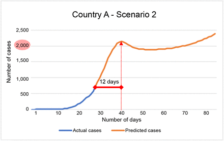
• Scenario 2: Moderate reductions (CIM=-3) on mobility for the first 2 weeks and then relaxed measures (CIM>0) moving forward. In low income economies, a balance between a lockdown and public health is needed, hence, authors suggest a 2-week projections as viable. Peak number of cases is about 2,100 cases and R_t=0.99 before mobility measures were relaxed below -80%, where number of cases started to increase over 5,000 cases. Figure 5 shows total number of cases and behavior over the time. This scenario illustrates a lack of monitoring in mobility causing the virus to spread again, with increased number of cases.

  

  • Download figure
  • Open in new tab

  Figure 5.

  Country A, Scenario 2 - Peak number of cases were around 2,100 cases on day 42 since first documented case or 12 days after the last know data. Number of cases would increase due to mobility measures relaxation after day 56 and on.

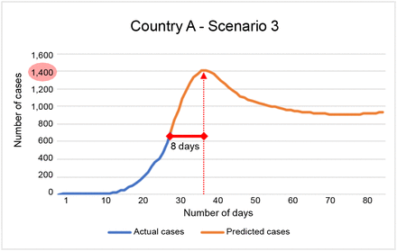
• Scenario 3: Strong reductions on mobility for the first 5 days (CIM=-5), moderate measures for the next 5 days (CIM=-3), and relaxed measures after 2 weeks. After the tenth day, R_t=0.98, peak number of cases is about 1,400 with a total reduction of mobility of -79.56%. On the projected eleventh day, people can start moving, hence a constant surveillance of R_t is needed to avoid cases growth as a result of increased mobility. Figure 6 shows total number of cases and behavior over the time.

  

  • Download figure
  • Open in new tab

  Figure 6.

  Country A, Scenario 3 - Peak number of cases were around 1,400 cases on day 38 since first documented case or 8 days after the last know data. Number of cases would increase due to mobility measures relaxation.

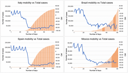
Looking into real data, a similar scenario 1 corresponds to a similar behavior show by Italy and Spain, both had apparently a good control in number of cases however, both had a large R_e for that period, more specifically a large R_e 14-day rolling average in the first 4 weeks. In order to achieve pandemic control, it was necessary to go to levels of 80% of mobility reduction over a period of 100 days in order to reach R_e<1, making economy practically to stop. This measure results inviable from economic and social perspectives plus the risk of crashing the health system as occurred unfortunately in both countries. Figure 7 shows the actual number of cases and needed CIM to decelerate pandemic wave.

• Download figure
• Open in new tab

Figure 7.

Italy and Spain behavior of number of cases and CIM.

In contrast, countries like Mexico and Brazil, which still show a growing behavior, even both have strong correlations, the difference is in the second 14-day period for number of cases. Mexico had around 500 cases whereas Brazil had almost 2000 cases in the same period of time. It can be expected that mobility reductions in Brazil might be stronger than Mexico ones. Figure 7 also shows the pandemic curves and their CIM.

6. Conclusions

In this article it was described the impact on mobility reductions in the public space as a measure to stop the pandemic wave of SARS-COV-2 virus. Also it was discussed mobility reductions as a way to project potential scenarios depending upon a variable called CIM as a method to monitor cases growth but also to control them. Three scenarios were discussed:

• Light measures, large number of cases, heavy mobility reductions, several impact on economies.

• Moderate measures, manageable number of cases, risk to case growth if not surveillance is applied with potential impact on public health system.

• Strong measures, reduced number of cases, manageable reduction on mobility and constant surveillance of cases to manage mobility recommendations. Public health system is not affected nor local economies.

As discussed, countries like Spain and Italy had to practically stop their economies in order to stop virus spread crashing their public health systems due to a poor surveillance program to monitor virus spread and mobility reductions. 60 days projections for US might anticipate heavy growing by observing their negative correlation and actual number of cases validate the impact on mobility. For Brazil, it can be anticipated that even its strong correlation, initial 30 days case growth will impact future case growth, making mobility measures much stronger.

Four main takeaways are made after all this analysis:

1. The importance of monitor case daily increase for the first 4-6 weeks of the pandemic is crucial to determine reduction in mobility and proper actions.

2. Any 2-digit increase in R_e will result in heavy case growth if mobility is not reduced as early as possible at levels to at least -20%.

3. m₀ parameter is determined by two factors: mobility reduction change and phase in the pandemic wave, the earliest, the better. Every 1% reduction in m₀ is variable depending upon the trend of CIM and R_t reductions but is in the range of 0.1 and 0.005 for every 1% of CIM. The earliest identification on case increase will require less mobility reductions.

4. A balance between stronger mobility reduction measures and lighter ones depends on R_t value and pandemic wave phase (an indirect variable of number of cases as described). CIM reduction can be in the range of -20% up to -80%.

7. Author contribution statement

Morales-Fajardo: Conceptualization, Methodology, Formal analysis, Investigation, Writing - Original Draft.

Rodríguez-Arce: Conceptualization, Methodology, Writing - Original Draft.

Funding

No external funding.

Declaration of competing interest

None.