
Abstract
Within days of first detection, Omicron SARS-CoV-2 variant case numbers grew exponentially and spread globally. To better understand variant epidemiological characteristics, we utilize a model-inference system to reconstruct SARS-CoV-2 transmission dynamics in South Africa and decompose novel variant transmissibility and immune erosion. Accounting for under-detection of infection, infection seasonality, nonpharmaceutical interventions, and vaccination, we estimate that the majority of South Africans had been infected by SARS-CoV-2 before the Omicron wave. Based on findings for Gauteng province, Omicron is estimated 100.3% (95% CI: 74.8 - 140.4%) more transmissible than the ancestral SARS-CoV-2 and 36.5% (95% CI: 20.9 - 60.1%) more transmissible than Delta; in addition, Omicron erodes 63.7% (95% CI: 52.9 - 73.9%) of the population immunity, accumulated from prior infections and vaccination, in Gauteng.
Main text
In late November, 2021, South African scientists and public health officials reported a new SARS-CoV-2 variant, subsequently named Omicron.1 Within days, SARS-CoV-2 cases due to Omicron increased dramatically in several provinces in South Africa,2 despite substantial prior infection of the population during previous pandemic waves, including a large, recent Delta wave. Concurrently, Omicron was detected in an increasing number of countries (89, as of 12/17/21; GISAID data3) and appeared to spread with unprecedented speed in several European countries.4,5 Multiple laboratory studies have reported large reductions (∼20-40x) in neutralizing ability of convalescent sera and vaccinee sera against Omicron, suggesting this variant is able to erode components of adaptive immunity.6-9 In addition, preliminary in vitro and/or ex vivo studies indicate that Omicron replicates faster within host than the Delta SARS-CoV-2 variant,8,10 which has been the predominant variant since mid 2021. Together, this early epidemiological and laboratory evidence points to both immune erosion and increased transmissibility of Omicron. However, the relative importance of these two quantities remains unclear.
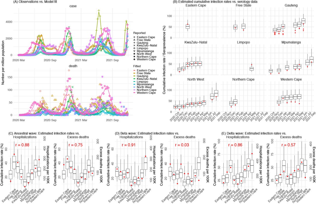
To better understand the epidemiological characteristics of Omicron, we utilize a model-inference system similar to one developed for study of SARS-CoV-2 variants of concern (VOCs), including the Beta variant.11 We use this system first to reconstruct SARS-CoV-2 transmission dynamics in each of the nine provinces in South Africa, accounting for under-detection of infection, infection seasonality, implemented nonpharmaceutical interventions (NPIs), and vaccination (see Methods). Overall, the model-inference system is able to fit weekly case and death data in each province (Fig 1A and Fig S1). We further validated the model-inference estimates using three independent datasets. First, we used serology data. We note that early in the pandemic serology data may reflect underlying infection rates but later, due to waning antibody titers and reinfection, likely underestimate infection. Compared to seroprevalence measures taken at multiple time points in each province, our model estimated cumulative infection rates roughly match corresponding serology measures and trends over time; as expected, model estimates were higher than serology measures taken during later months (Fig 1B). Second, compared to hospital admission data, across the nine provinces, model estimated infection numbers were well correlated with numbers of hospitalizations for all three initial pandemic waves caused by the ancestral, Beta, and Delta variants, respectively (r > .85, Fig 1 C-E). Third, model-estimated infection numbers were correlated with age-adjusted excess mortality for both the ancestral and Delta wave, but not the Beta wave (Fig 1C and E, vs. Fig 1D). Overall, these comparisons indicate our model-inference estimates align with underlying transmission dynamics.

Pandemic dynamics in each of the nine provinces (see legend); dots depict reported weekly numbers of cases and deaths; lines show model mean estimates (in the same color). For validation, model estimated infection rates are compared to seroprevalence measures over time from multiple sero-surveys summarized in ref 1 (B), COVID-related hospitalizations (left panel) and age-adjusted excess mortality (right panel) during the Ancestral (C), Beta (D), and Delta (E) waves. Boxplots depict the estimated distribution for each province (middle bar = mean; edges = 50% CrIs) and whiskers (95% CrIs). Red dots show corresponding measurements. Correlation (r) between model estimated cumulative infection rate and cumulative hospitalization or age-adjusted excess mortality (C-E) for each wave is shown in each plot. Note that hospitalization data begin from 6/6/20 and excess mortality data begin from 5/3/20 and thus are incomplete for the Ancestral wave.
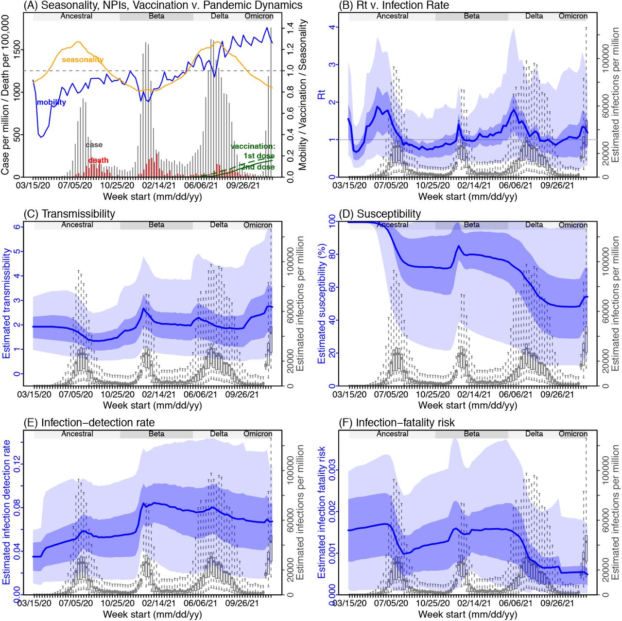
Next, we use Gauteng – the province with the earliest surge of Omicron – as an example to highlight pandemic dynamics in South Africa thus far and develop key model-inference estimates (Fig 2 for Gauteng and Fig S 2-9 for each of the other eight provinces). Despite lower cases per capita than many other countries, infection numbers in South Africa were likely much higher due to under-detection. For Gauteng, the estimated infection-detection rate during the first pandemic wave was 4.31% (95% CI: 2.53 - 8.75%), and increased slightly to 5.21% (95% CI: 2.94 - 9.47%) and 5.88% (95% CI: 3.40 - 11.32%) during the Beta and Delta waves, respectively (Table S1). These estimates are in line with those reported elsewhere based on serology data (e.g., 4.74% detection rate during the first wave12). Accounting for under-detection (Fig 2E), we estimate that 34.99% (95% CI: 17.22 - 59.52%, Table S2) of the population in Gauteng were infected during the first wave, predominantly during winter when more conducive climate conditions and relaxed public health restrictions existed (see the estimated seasonal and mobility trends, Fig 2A).

(A) Observed relative mobility, vaccination rate, and estimated disease seasonal trend, compared to case and death rates over time. Key model-inference estimates are shown for the time-varying effective reproduction number Rt (B), transmissibility (C), population susceptibility (D), infection-detection rate (E), and infection-fatality risk (F). Grey shaded areas indicate the approximate circulation period for each variant. In (B) – (F), blue lines and surrounding areas show the estimated mean, 50% (dark) and 95% (light) CrIs; boxes and whiskers show the estimated mean, 50% and 95% CrIs for estimated infection rates. Note that the transmissibility estimates (in C) have removed the effects of changing population susceptibility, NPIs, and disease seasonality; thus, the trends are more stable than the reproduction number (Rt in B) and reflect changes in variant-specific properties. Also note that infection-fatality risk estimates were based on reported COVID-19 deaths and may not reflect true values due to likely under-reporting of COVID-19 deaths.
With the emergence of Beta, another 25.91% (95% CI: 14.26 - 45.91%) of the population in Gauteng – including reinfections – is estimated to have been infected, even though the Beta wave occurred during summer under less conducive climate conditions for transmission (Fig 2A). Consistent with laboratory studies showing low neutralizing ability of convalescent sera against Beta,13,14 the model-inference system estimates a large increase in population susceptibility with the surge of Beta (Fig 2D). In addition to this immune erosion, an increase in transmissibility is also evident for Beta, after accounting for concurrent NPIs and infection seasonality (Fig 2C). Notably, in contrast to the large fluctuation of the time-varying effective reproduction number over time (Rt, Fig 2B), the transmissibility estimates are more stable and reflect changes in variant-specific properties. Further, consistent with in-depth epidemiological findings,15 the estimated overall infection-fatality risk was higher for Beta than Ancestral SARS-CoV-2 (0.16% [95% CI: 0.09 - 0.28%] vs. 0.09% [95% CI: 0.05 - 0.18%], Fig 2F and Table S3; n.b. these estimates are based on documented COVID-19 deaths and are likely underestimates).
With the introduction of Delta, a third pandemic wave occurred in Gauteng during the 2021 winter. The model-inference system estimates a 53.19% (95% CI: 27.61 - 91.87%) attack rate by Delta, despite the large number of infections during the previous two waves. This large attack rate was possible, due to the high transmissibility of Delta, as reported in multiple studies,16-20 the more conducive winter transmission conditions (Fig 2A), and the immune erosion from Delta relative to both the ancestral and Beta variants. Consistent with this finding, and in particular the estimated immune erosion, studies have reported a 27.5% reinfection rate during the Delta pandemic wave in Delhi, India21 and reduced ability of sera from Beta-infection recoverees to neutralize Delta.22,23
Due to these large pandemic waves, prior to the detection of Omicron in Gauteng, estimated cumulative infection numbers surpassed the population size (Fig 3B), indicating the large majority of the population had been infected and some more than once. With the rise of Omicron, the model-inference system estimates a very large increase in population susceptibility (Fig 2D), as well as an increase in transmissibility (Fig 2C); however, unlike previous waves, the Omicron wave progresses much more quickly, peaking 2-3 weeks after initiating marked exponential growth. These estimates suggest that several additional factors may have also contributed to the observed dynamics, including changes to the infection-detection rate (Fig 2E), a summer seasonality increasingly suppressing transmission as the wave progresses (Fig 2A), as well as a slight change in population mobility suggesting potential behavior changes (Fig 2A).

Heatmaps show (A) Estimated mean infection rates by week (x-axis) and province (y-axis), (B) Estimated mean cumulative infection numbers relative to the population size in each province, and (C) Estimated population susceptibility (to the circulating variant) by week and province. Boxplots in the top row show the estimated distribution of changes in transmissibility for Beta, Delta, and Omicron, relative to the Ancestral SARS-CoV-2, for each province (middle bar = median; edges = 50% CIs; and whiskers =95% CIs); boxplots in the bottom row show, for each variant, the estimated distribution of immune erosion to all adaptive immunity gained from infection and vaccination prior to that variant. Red lines show the mean across all provinces. Estimates for Omicron are not shown for some provinces, as data were not sufficient for model inference.
Across all nine provinces in South Africa, the pandemic timing and intensity varied (Fig 3 A-C). In addition to Gauteng, high cumulative infection rates during the first three pandemic waves are also estimated for Western Cape and Northern Cape (Fig 1 C-E, Fig 3B and Table S2). Overall, all nine provinces likely experienced three large pandemic waves prior to the growth of Omicron; estimated average cumulative infections ranged from 58% of the population in Limpopo to 126% in Northern Cape (Fig 3B).
Combining these model-inference estimates during each wave in each province, we estimate that Beta eroded immunity among 72.1% (95% CI: 52.8 - 88.6%) of individuals with prior ancestral SARS-CoV-2 infection and was 38.5% (95% CI: 16.2 – 56.0%) more transmissible than the ancestral SARS-CoV-2. These estimates for Beta are consistent across the nine provinces (Fig 3D, 1st column), as well as with our previous estimates using national data for South Africa.11 In comparison, estimates for Delta vary across the nine provinces (Fig 3D, 2nd column), given the more diverse population immune landscape among provinces after two pandemic waves. Overall, we estimate that Delta eroded 32.5% (95% CI: 0 – 60.9%) of prior immunity (gained from infection by ancestral SARS-CoV-2 and/or Beta, and/or vaccination) and was 38.3% (95% CI: 21.2 - 58.5%) more transmissible than the ancestral SARS-CoV-2.
For Omicron, based on three provinces with the earliest surges (i.e., Gauteng, North West, and Western Cape), we estimate that this variant erodes 55.0% (95% CI: 40.9 - 71.4%) of immunity due to all prior infections and vaccination. In addition, it is 92.2% (95% CI: 70.2 - 128.5%) more transmissible than the ancestral SARS-CoV-2. Based on estimates for Gauteng alone, Omicron is 100.3% (95% CI: 74.8 - 140.4%) more transmissible than the ancestral SARS-CoV-2, and 36.5% (95% CI: 20.9 - 60.1%) more transmissible than Delta; in addition, it erodes 63.7% (95% CI: 52.9 - 73.9%) of the population immunity, accumulated from prior infections and vaccination, in Gauteng.
Using a comprehensive model-inference system, we have reconstructed the pandemic dynamics in each of the nine provinces in South Africa. Estimated underlying infection rates (Fig 1B-E) and key parameters (e.g. infection-detection rate and infection-fatality risk) are in line with independent epidemiological data and investigations. These detailed model-inference estimates thus allow assessment of both the transmissibility and immune erosion potential of Omicron, and help contextualization and interpretation of Omicron transmission dynamics in places outside South Africa. We show that, prior to the rise of Omicron, in Gauteng, the large majority of population had been infected by one or more SARS-CoV-2 variants (including the ancestral virus, Beta, and Delta), suggesting a high rate of immune erosion by Omicron versus most, if not all, prior SARS-CoV-2 variants and vaccines. Interestingly, preliminary laboratory data show that only 1 of 8 Beta, 1 of 7 Delta, and 0 of 10 Alpha convalescent sera had 50% neutralization titers (IC50) >1:16 for Omicron.9 Combining these laboratory data with our estimates of infection rates suggests 11% of the population would have retained immunity against Omicron from prior Beta and Delta infection (i.e., 1/8 × 25.9% attack rate by Beta + 1/7 × 53.2% attack rate by Delta). However, studies have reported retained neutralizing ability against Omicron among recoverees additionally vaccinated with 2 doses of vaccine.7,9 Assuming an 80% probability of prior infection among the ∼25% of Gauteng who received at least 1 vaccine dose (by the end of Nov 2021), another 20% of population would have gained immunity against Omicron from infection plus vaccination. In combination, this simple conversion suggests the remaining ∼70% of the population would be susceptible to Omicron, similar to our model estimates (Fig 2D). Given the challenge of jointly estimating population susceptibility (needed for estimating both prior immunity and immune erosion) and transmissibility, the consistency of our population susceptibility estimates with available laboratory evidence indicates that our estimates of transmissibility are also sensible.
Population susceptibility may differ across locations depending upon prior exposure to different SARS-CoV-2 variants and vaccination uptake. However, similar calculations can be made in other countries and regions, given prior infection and vaccination rates, in order to gauge local susceptibility. In combination with the increased transmissibility estimated here and other location conditions (e.g., infection seasonality and implementation of NPIs), modeling can then be used to better anticipate the course of the Omicron wave. Nonetheless, the ability of Omicron to spread with unprecedented pace in a heavily infected and partially vaccinated population should serve as an alert for prompt public health response. More fundamentally, it is yet another indication of the need for a global effort for increased vaccination, recurrent boosting, and the development and distribution of effective and safe therapeutics for all populations around the world.
METHODS
Data sources and processing
We used reported COVID-19 case and mortality data to capture transmission dynamics, weather data to estimate infection seasonality, mobility data to represent concurrent NPIs, and vaccination data to account for changes in population susceptibility due to vaccination in the model-inference system. Provincial level COVID-19 case, mortality, and vaccination data were sourced from the Coronavirus COVID-19 (2019-nCoV) Data Repository for South Africa (COVID19ZA).24 Hourly surface station temperature and relative humidity came from the Integrated Surface Dataset (ISD) maintained by the National Oceanic and Atmospheric Administration (NOAA) and are accessible using the “stationaRy” R package.25,26 We computed specific humidity using temperature and relative humidity per the Clausius-Clapeyron equation.27 We then aggregated these data for all weather stations in each province with measurements since 2000 and calculated the average for each week of the year during 2000-2020.
Mobility data were derived from Google Community Mobility Reports;28 we aggregated all business-related categories (i.e., retail and recreational, transit stations, and workplaces) in all locations in each province to weekly intervals. For vaccination, provincial vaccination data from the COVID19ZA data repository recorded the total number of vaccine doses administered over time; to obtain a breakdown for numbers of partial (1 dose of mRNA vaccine) and full vaccinations (1 dose of Janssen vaccine or 2 doses of mRNA vaccine), separately, we used national vaccination data for South Africa from Our World in Data29,30 to apportion the doses each day. In addition, cumulative case data suggested 18,586 new cases on Nov 23, 2021, whereas the South Africa Department of Health reported 868.31 Thus, for Nov 23, 2021, we used linear interpolation to fill in estimates for each province on that day and then scaled the estimates such that they sum to 868.
Model-inference system
The model-inference system is based on our previous work estimating changes in transmissibility and immune erosion for SARS-CoV-2 VOCs including Alpha, Beta, Gamma, and Delta.11,32 Below we describe each component.
Epidemic model
The epidemic model follows an SEIRSV (susceptible-exposed-infectious-recovered-susceptible-vaccination) construct per Eqn 1:
 where S, E, I, R are the number of susceptible, exposed (but not yet infectious), infectious, and recovered/immune/deceased individuals; N is the population size; and ε is the number of travel-imported infections. In addition, the model includes the following key components:
Virus-specific properties, including the time-varying variant-specific transmission rate βt, latency period Zt, infectious period Dt, and immunity period Lt. Note all parameters are estimated for each week (t) as described below.
The impact of NPIs. Specifically, we use relative population mobility (see data above) to adjust the transmission rate via the term mt, as the overall impact of NPIs (e.g., reduction in the time-varying effective reproduction number Rt) has been reported to be highly correlated with population mobility during the COVID-19 pandemic.33-35 To further account for potential changes in effectiveness, the model additionally includes a parameter, et, to scale NPI effectiveness.
The impact of vaccination, via the terms v1,t and v2,t. Specifically, v1,t is the number of individuals successfully immunized after the first dose of vaccine and is computed using vaccination data and vaccine effectiveness (VE) for 1st dose; and v2,t is the additional number of individuals successfully immunized after the second vaccine dose (i.e., excluding those successfully immunized after the first dose). In South Africa, around two-thirds of vaccines administered during our study period were the mRNA BioNTech/Pfizer vaccine and one-third the Janssen vaccine.36 We thus set VE to 20%/85% (partial/full vaccination) for Beta, 35%/75% for Delta, and 10%/35% for Omicron based on reported VE estimates.37-39
Infection seasonality, computed using temperature and specific humidity data as described previously (see supplemental material of Yang and Shaman11). Briefly, we estimated the relative seasonal trend (bt) using a model representing the dependency of the survival of respiratory viruses including SARS-CoV-2 to temperature and humidity.40,41 As shown in Fig 2A, bt estimates over the year averaged to 1 such that weeks with bt >1 (e.g. during the winter) are more conducive to SARS-CoV-2 transmission whereas weeks with bt <1 (e.g. during the summer) have less favorable climate conditions for transmission. The estimated relative seasonal trend, bt, is used to adjust the relative transmission rate at time t in Eqn 1.
Observation model to account for under-detection and delay
Using the model-simulated number of infections occurring each day, we further computed the number of cases and deaths each week to match with the observations, as done in Yang et al.42 Briefly, we include 1) a time-lag from infectiousness to detection (i.e., an infection being diagnosed as a case), drawn from a gamma distribution with a mean of Td,mean days and a standard deviation of Td, sd days, to account for delays in detection (Table S4); 2) an infection-detection rate (rt), i.e. the fraction of infections (including subclinical or asymptomatic infections) reported as cases, to account for under-detection; 3) a time-lag from infectiousness to death, drawn from a gamma distribution with a mean of 13-15 days and a standard deviation of 10 days; and 4) an infection-fatality risk (IFRt). To compute the model-simulated number of new cases each week, we multiplied the model-simulated number of new infections per day by the infection-detection rate, and further distributed these simulated cases in time per the distribution of time-from-infectiousness-to-detection. Similarly, to compute the model-simulated deaths per week and account for delays in time to death, we multiplied the simulated-infections by the IFR and then distributed these simulated deaths in time per the distribution of time-from-infectious-to-death. We then aggregated these daily numbers to weekly totals to match with the weekly case and mortality data for model-inference. For each week, the infection-detection rate (rt), the infection-fatality risk (IFRt)., and the two time-to-detection parameters (Td,mean and Td, sd) were estimated along with other parameters (see below).
Model inference and parameter estimation
The inference system uses the ensemble adjustment Kalman filter, EAKF,43 a Bayesian statistical method, to estimate model state variables (i.e., S, E, I, R from Eqn 1) and parameters (i.e.,αt, Zt, Dt, Lt, et, from Eqn 1 as well as rt, IFRt and other parameters from the observation model). Briefly, the EAKF uses an ensemble of model realizations (n=500 here), each with initial parameters and variables randomly drawn from a prior range (see Table S4). After model initialization, the system integrates the model ensemble forward in time for a week (per Eqn 1) to compute the prior distribution for each model state variable and parameter, as well as the model-simulated number of cases and deaths for that week. The system then combines the prior estimates with the observed case and death data for the same week to compute the posterior per Bayes’ theorem.43 During this filtering process, the system updates the posterior distribution of all model variables and parameters for each week.
Estimating changes in transmissibility and immune erosion for each variant
As in ref11, we computed the variant-specific transmissibility (RTX) as the product of the variant-specific transmission rate (βt) and infectious period (Dt). Note that Rt, the time-varying effective reproduction number, is defined as Rt = btetmtβtDtS/N = btetmtRTXS/N. To reduce uncertainty, we averaged transmissibility estimates over the period a particular variant of interest was predominant. To find these predominant periods, we first specified the approximate timing of each pandemic wave in each province based on: 1) when available, genomic surveillance data; specifically, the onsets of the Beta wave in Eastern Cape, Western Cape, KwaZulu-Natal, and Northern Cape, were separately based on the initial detection of Beta in these provinces as reported in Tegally et al;44 the onsets of the Delta wave in each of the nine provinces, separately, were based on genomic sequencing data from the Network for Genomic Surveillance South Africa (NGS-SA);45 and 2) when genomic data were not available, we used the week with the lowest case number between two waves. The specified calendar periods are listed in Table S5. During later waves, multiple variants could initially co-circulate before one became predominant. As a result, the estimated transmissibility tended to increase before reaching a plateau (see, e.g., Fig 2C). In addition, in a previous study of the Delta pandemic wave in India,32 we also observed that when many had been infected, transmissibility could decrease a couple months after the peak, likely due to increased reinfections for which onward transmission may be reduced. Thus, to obtain a more variant-specific estimate, we computed the average transmissibility  using the weekly RTX estimates over the 8-week period starting the week prior to the maximal Rtx during each wave; if no maximum existed (e.g. when a new variant is less transmissible), we simply averaged over the entire wave. We then computed the change in transmissibility due to a given variant relative to the ancestral SARS-CoV-2 as
 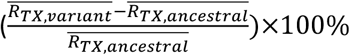 .
.
Approximate epidemic timing for each wave in each province.
To quantify immune erosion, similar to ref11, we estimated changes in susceptibility over time and computed the change in immunity as ΔImm = St+1 – St + it, where St is the susceptibility at time-t and it is the new infections occurring during each week-t. We sum over all ΔImm estimates for a particular location, during each wave, to compute the total change in immunity due to a new variant, ΣΔImmv. We then computed the level of immune erosion as the ratio of ΣΔImmv to the model-estimated population immunity prior to the first detection of immune erosion, during each wave. That is, as opposed to having a common reference of prior immunity, here immune erosion for each variant depends on the state of the population immune landscape – i.e., combining all prior exposures and vaccinations – immediately preceding the surge of that variant.
For all provinces, model-inference was initiated the week starting March 15, 2020 and run continuously until the week starting Dec 12, 2021. To account for model stochasticity, we repeated the model-inference process 100 times for each province, each with 500 model realizations and summarized the results from all 50,000 model estimates.
Model validation using independent data
To compare model estimates with independent observations not assimilated into the model-inference system, we utilized three relevant datasets:
Serological survey data measuring the prevalence of SARS-CoV-2 antibodies over time. Multiple serology surveys have been conducted in different provinces of South Africa. The South African COVID-19 Modelling Consortium summarizes the findings from several of these surveys (see Fig 1A of ref 46). We digitized all data presented in Fig 1A of ref 46 and compared these to corresponding model-estimated cumulative infection rates (computed mid-month for each corresponding month with a seroprevalence measure). Due to unknown survey methodologies and challenges adjusting for sero-reversion and reinfection, we used these data directly (i.e., without adjustment) for qualitative comparison.
COVID-19-related hospitalization data, from COVID19ZA.24 We aggregated the total number of COVID-19 hospital admissions during each wave and compared these aggregates to model-estimated cumulative infection rates during the same wave. Of note, these hospitalization data were available from June 6, 2020 onwards and are thus incomplete for the first wave.
Age-adjusted excess mortality data from the South African Medical Research Council (SAMRC).47 Deaths due to COVID-19 (used in the model-inference system) are undercounted. Thus, we also compared model-estimated cumulative infection rates to age-adjusted excess mortality data during each wave. Of note, excess mortality data were available from May 3, 2020 onwards and are thus incomplete for the first wave.
Code availability
All source code and data necessary for the replication of our results and figures will be made publicly available on Github.
Author contributions
WY designed the study (main), conducted the model analyses, interpreted results, and wrote the first draft. JS designed the study (supporting), interpreted results, and critically revised the manuscript.
Competing interests
JS and Columbia University disclose partial ownership of SK Analytics. JS discloses consulting for BNI.
Supplemental Figures and Tables

Model-fit to case and death data in each province. Dots show reported SARS-CoV-2 cases and deaths by week. Blue lines and surrounding area show model estimated median, 50% (darker blue) and 95% (lighter blue) credible intervals.

(A) Observed relative mobility, vaccination rate, and estimated disease seasonal trend, compared to case and death rates over time. Key model-inference estimates are shown for the time-varying effective reproduction number Rt (B), transmissibility (C), population susceptibility (D), infection-detection rate (E), and infection-fatality risk (F). Grey shaded areas indicate the approximate circulation period for each variant. In (B) – (F), blue lines and surrounding areas show the estimated mean, 50% (dark) and 95% (light) CrIs; boxes and whiskers show the estimated mean, 50% and 95% CrIs for estimated infection rates. Note that the transmissibility estimates (in C) have removed the effects of changing population susceptibility, NPIs, and disease seasonality; thus, the trends are more stable than the reproduction number (Rt in B) and reflect changes in variant-specific properties. Also note that infection-fatality risk estimates were based on reported COVID-19 deaths and may not reflect true values due to likely under-reporting of COVID-19 deaths.
(A) Observed relative mobility, vaccination rate, and estimated disease seasonal trend, compared to case and death rates over time. Key model-inference estimates are shown for the time-varying effective reproduction number Rt (B), transmissibility (C), population susceptibility (D), infection-detection rate (E), and infection-fatality risk (F). Grey shaded areas indicate the approximate circulation period for each variant. In (B) – (F), blue lines and surrounding areas show the estimated mean, 50% (dark) and 95% (light) CrIs; boxes and whiskers show the estimated mean, 50% and 95% CrIs for estimated infection rates. Note that the transmissibility estimates (in C) have removed the effects of changing population susceptibility, NPIs, and disease seasonality; thus, the trends are more stable than the reproduction number (Rt in B) and reflect changes in variant-specific properties. Also note that infection-fatality risk estimates were based on reported COVID-19 deaths and may not reflect true values due to likely under-reporting of COVID-19 deaths.
(A) Observed relative mobility, vaccination rate, and estimated disease seasonal trend, compared to case and death rates over time. Key model-inference estimates are shown for the time-varying effective reproduction number Rt (B), transmissibility (C), population susceptibility (D), infection-detection rate (E), and infection-fatality risk (F). Grey shaded areas indicate the approximate circulation period for each variant. In (B) – (F), blue lines and surrounding areas show the estimated mean, 50% (dark) and 95% (light) CrIs; boxes and whiskers show the estimated mean, 50% and 95% CrIs for estimated infection rates. Note that the transmissibility estimates (in C) have removed the effects of changing population susceptibility, NPIs, and disease seasonality; thus, the trends are more stable than the reproduction number (Rt in B) and reflect changes in variant-specific properties. Also note that infection-fatality risk estimates were based on reported COVID-19 deaths and may not reflect true values due to likely under-reporting of COVID-19 deaths.

(A) Observed relative mobility, vaccination rate, and estimated disease seasonal trend, compared to case and death rates over time. Key model-inference estimates are shown for the time-varying effective reproduction number Rt (B), transmissibility (C), population susceptibility (D), infection-detection rate (E), and infection-fatality risk (F). Grey shaded areas indicate the approximate circulation period for each variant. In (B) – (F), blue lines and surrounding areas show the estimated mean, 50% (dark) and 95% (light) CrIs; boxes and whiskers show the estimated mean, 50% and 95% CrIs for estimated infection rates. Note that the transmissibility estimates (in C) have removed the effects of changing population susceptibility, NPIs, and disease seasonality; thus, the trends are more stable than the reproduction number (Rt in B) and reflect changes in variant-specific properties. Also note that infection-fatality risk estimates were based on reported COVID-19 deaths and may not reflect true values due to likely under-reporting of COVID-19 deaths.

(A) Observed relative mobility, vaccination rate, and estimated disease seasonal trend, compared to case and death rates over time. Key model-inference estimates are shown for the time-varying effective reproduction number Rt (B), transmissibility (C), population susceptibility (D), infection-detection rate (E), and infection-fatality risk (F). Grey shaded areas indicate the approximate circulation period for each variant. In (B) – (F), blue lines and surrounding areas show the estimated mean, 50% (dark) and 95% (light) CrIs; boxes and whiskers show the estimated mean, 50% and 95% CrIs for estimated infection rates. Note that the transmissibility estimates (in C) have removed the effects of changing population susceptibility, NPIs, and disease seasonality; thus, the trends are more stable than the reproduction number (Rt in B) and reflect changes in variant-specific properties. Also note that infection-fatality risk estimates were based on reported COVID-19 deaths and may not reflect true values due to likely under-reporting of COVID-19 deaths.

(A) Observed relative mobility, vaccination rate, and estimated disease seasonal trend, compared to case and death rates over time. Key model-inference estimates are shown for the time-varying effective reproduction number Rt (B), transmissibility (C), population susceptibility (D), infection-detection rate (E), and infection-fatality risk (F). Grey shaded areas indicate the approximate circulation period for each variant. In (B) – (F), blue lines and surrounding areas show the estimated mean, 50% (dark) and 95% (light) CrIs; boxes and whiskers show the estimated mean, 50% and 95% CrIs for estimated infection rates. Note that the transmissibility estimates (in C) have removed the effects of changing population susceptibility, NPIs, and disease seasonality; thus, the trends are more stable than the reproduction number (Rt in B) and reflect changes in variant-specific properties. Also note that infection-fatality risk estimates were based on reported COVID-19 deaths and may not reflect true values due to likely under-reporting of COVID-19 deaths.

(A) Observed relative mobility, vaccination rate, and estimated disease seasonal trend, compared to case and death rates over time. Key model-inference estimates are shown for the time-varying effective reproduction number Rt (B), transmissibility (C), population susceptibility (D), infection-detection rate (E), and infection-fatality risk (F). Grey shaded areas indicate the approximate circulation period for each variant. In (B) – (F), blue lines and surrounding areas show the estimated mean, 50% (dark) and 95% (light) CrIs; boxes and whiskers show the estimated mean, 50% and 95% CrIs for estimated infection rates. Note that the transmissibility estimates (in C) have removed the effects of changing population susceptibility, NPIs, and disease seasonality; thus, the trends are more stable than the reproduction number (Rt in B) and reflect changes in variant-specific properties. Also note that infection-fatality risk estimates were based on reported COVID-19 deaths and may not reflect true values due to likely under-reporting of COVID-19 deaths.

(A) Observed relative mobility, vaccination rate, and estimated disease seasonal trend, compared to case and death rates over time. Key model-inference estimates are shown for the time-varying effective reproduction number Rt (B), transmissibility (C), population susceptibility (D), infection-detection rate (E), and infection-fatality risk (F). Grey shaded areas indicate the approximate circulation period for each variant. In (B) – (F), blue lines and surrounding areas show the estimated mean, 50% (dark) and 95% (light) CrIs; boxes and whiskers show the estimated mean, 50% and 95% CrIs for estimated infection rates. Note that the transmissibility estimates (in C) have removed the effects of changing population susceptibility, NPIs, and disease seasonality; thus, the trends are more stable than the reproduction number (Rt in B) and reflect changes in variant-specific properties. Also note that infection-fatality risk estimates were based on reported COVID-19 deaths and may not reflect true values due to likely under-reporting of COVID-19 deaths.
Numbers show the estimated percentage of infections (including asymptomatic and subclinical infections) documented as cases (mean and 95% CI in parentheses).
Numbers show estimated cumulative infection numbers, expressed as percentage of population size (mean and 95% CI in parentheses).
Numbers are percentages (%; mean and 95% CI in parentheses). Note that these estimates were based on reported COVID-19 deaths and may be biased due to likely under-reporting of COVID-19 deaths.
Prior ranges for the parameters used in the model-inference system.
Acknowledgements
This study was supported by the National Institute of Allergy and Infectious Diseases (AI145883 and AI163023), the Centers for Disease Control and Prevention (CK000592), and a gift from the Morris-Singer Foundation.
References


