Abstract
Many countries hit by the COVID-19 epidemic consider the introduction of vaccination passes. So far, no thorough impact assessment of vaccination passes and of lower restrictions for their holders has been conducted. Here, we propose the VAP-SIRS model that accounts for susceptible, infected, and recovered subpopulations, also within the group of vaccinated pass holders. The model accounts for imperfect vaccination effectiveness, revaccinations and waning immunity. Different restrictions for pass holders and the rest of the population result in different scenarios of the epidemic evolution, some of which yield unfavourable COVID-19 dynamics and new waves. We identify critical variables that should be considered by policymakers and show how unfavourable outcomes can be avoided using adaptive policies. In particular, while pass holders could initially be allowed large freedoms, the gradual loss of immunity will require either increased restrictions for pass holders, or accelerated revaccination. In the long-term, common restrictions for both the pass holders and the rest of the population will have to be kept to avoid epidemic resurgence. Such minimum required restrictions depend on vaccination effectiveness, revaccination rate, waning rate and fraction of never-vaccinated population, and, for realistic combinations of these parameters, range between 29% and 69% reduction of contacts.
Main
In the past, governments have required proof of vaccination for travel, with yellow fever being the best-known example, and the only disease for which a certificate is needed to cross borders in compliance to the International Health Regulations1. However, the idea that proof of vaccination will become a prerequisite for crossing borders or to enter facilities, visit businesses premises, participate in events, and generally enjoy more freedom, has only arisen in the context of combatting the COVID-19 epidemic. Despite technical challenges, scientific uncertainties, and ethical and legal dilemmas, the idea of vaccination passes (VPs), i.e., documents issued on the basis of vaccination status, is now receiving unprecedented attention2,3,4. Many consider VPs as tools to restore people’s freedoms and increase well-being, whilst allowing economies to reopen. Determining immunity status is challenging, as the immune response and its duration may greatly vary; this being applicable to post-vaccination immunity, as well as following natural SARS-CoV-2 infection and recovery5. It is, therefore, critically important to determine levels of restrictions that offer safety whilst being tolerable, ensuring good compliance and rational behaviour. Less than perfect conferred protection coupled with suboptimal levels of restrictions can have detrimental effects. The lack of a comprehensive framework to determine such levels, including when approaching higher vaccination coverage and even herd immunity, may result in policymakers opting to select suboptimal levels of restrictions. This may happen for different reasons, such as lack of true understanding of the ramifications, to boost morale or, even, for political gain. Evidence indicates vaccine effectiveness can greatly vary6,7 and it may be compromised due to escape variants8 and waning immunity9,10,11,12.
Various models have been developed to inform vaccination strategies13,14,15,16,17,18,19,20,21. One such effort indicates lower vaccine effectiveness coupled with an increase in social contact among those vaccinated (behavioral compensation) may undermine vaccination effects, even without considering immunity waning22. So far, there has been no model to focus on the medium- and long-term impact of relaxing restrictions for VP holders, with due consideration to vaccine effectiveness, durability of response, and vaccine hesitancy. The proposed VAP-SIRS model delivers a systematic framework to assess key considerations for policymaking.
Results
The VAP-SIRS model of the impact of COVID-19 vaccination passes
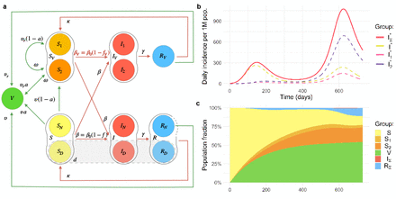
The VAP-SIRS model extends the classical SIRS model23 (red arrows in Fig. 1a) with additional states and parameters that describe the dynamics of vaccination routine in a population (green arrows in Fig 1a.). To this end, we consider the following subpopulations: (i) initially susceptible SN, who, if successfully vaccinated, populate the immune group V, with rate aυ, where υ is the vaccination rate and a is the effectiveness, (ii) susceptible who were vaccinated but did not gain immunity (S1), (iii) vaccinated, whose immunity waned with rate ω and became susceptible again (S2), (iv) susceptible, who are not and will never get vaccinated (SD). Additionally, revaccination of S2 populates V with rate aυr. All recovered, unless recovered compartment RD, are also subject to vaccination. The fraction of the population that will never be vaccinated is denoted d.
a. Graphical scheme of the VAP-SIRS model. b. The timeline of daily incidence per 1 million inhabitants for an effective vaccine (a = 0.9), slow (re-)vaccination rate (υ = υr = 0.004; typical for many European countries), proportional mixing (see Methods) and low fraction of never-vaccinated (d = 0.1). Here, a variable with the asterisk (*) indicates that we consider a daily incidence over the corresponding variable, thus I* stands for  , and by
  we mean the sum of all daily infected
  . c. The Muller plot of the population structure (the width of the color band in the y axis) as a function of time (x axis) for the same parameter settings as in b. Here, by IΣ and RΣ we denote I + IV and R + RV, respectively.
The presented model analysis is performed for carefully selected parameter setups: two different vaccination rates, 0.004 and 0.008 dose per person daily, chosen on the basis of the current rates observed in Europe24,25, and for vaccine effectivenesses 0.6 and 0.9, which conservatively model that of the most widely used vaccines: Vaxzevria (AstraZeneca)26,27 and Comirnaty (BioNTech/Pfizer)28,7,29, respectively. Furthermore, optimistic (500 days; ω = 1/500) and pessimistic (200 days; ω = 1/200) average immunity duration periods are considered, reflecting emerging data on large individual variation of immunity waning and other key factors influencing this process9,12,30,31,32. Finally, across the manuscript, we assume the revaccination rate υr = υ, and consider optimistic 0.1, and pessimistic 0.3 fractions of never-vaccinated d.
We assume that VP holders are all who were vaccinated at least once (Fig. 1). The restriction level f (ranging from 0 to 1) is introduced as a modulator of the SARS-CoV-2 reproduction number. Here, we consider that without any restrictions (f = 0), the reproduction number for the virus equals 4, as an optimistic estimate for B.1.1.733,34. Similarly, restrictions fv ≤ f for contacts among VP holders are considered. f and fv should be interpreted as the net effect of all factors that reduce the reproduction number of the virus within the respective groups: all applied non-pharmaceutical interventions together with the resulting changes in behavior. Based on the current studies, we fix the generation time to 6 days (γ = 1/6)34,33. Finally, we consider two types of mixing between subpopulations: proportional (typical for SIR models) and preferential, where the VP holders prefer contacts with other VP holders. See Methods for a detailed model description.
VAP-SIRS predicts a possible infection resurgence despite vaccinations
VAP-SIRS predicts unfavourable epidemic dynamics for a wide range of parameters. As an example consider: a = 0.9, υ = υr = 0.004, d = 0.1, and ω = 1/500, a seemingly safe setup, which we will call the reference setup. For such setup and low restrictions fv = 0.05 for VP holders as well as medium restrictions f = 0.63 for contacts with and within the rest of the population, the model predicts a small wave of infections shortly after the vaccination program starts, followed by a large wave later (Fig. 1b). This behavior is explained by the population structure and different restrictions (Fig. 1c). In this scenario, the first wave is driven by the unvaccinated susceptibles (SN) and suppressed by ongoing vaccination, as expected. Interestingly, the second, larger wave is driven by the SV group. The SV group is composed of the number of individuals for whom the vaccine was ineffective (S1) and those vaccinated who lose their immunity and are not yet revaccinated (S2). In the following we investigate how the dynamics change for different restrictions settings.
Stability analysis identifies potential scenarios for the COVID-19 epidemic depending on the restrictions imposed on VP holders and the rest of the population
To assess the epidemic evolution in different scenarios, we analysed stability by linearising the model equations with I = R = 0 (Methods). The restriction levels f = (f, fv) influence the instantaneous reproduction number R*. R*(t) is the reproduction number that would be observed at time t, given the restrictions f and the composition of the population, where the number of infected is very small. If R*(t) > 1, then switching to f at time t results in an overcritical epidemic evolution, with an initially exponential growth of infections; if R*(t) < 1, switching to f at time t results in a subcritical epidemic evolution, where the number of active cases decreases to zero. The R* is more informative of epidemic thresholds than the standard effective reproduction number, as it does not depend on the actual number of infected and recovered.
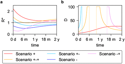
We consider five restriction choices (prototypical for five regions of the parameter space), leading to different time profiles of R* (Fig. 2a). Medium restrictions for both VP holders and the rest of the population (red curve in Fig. 2a) lead to an overcritical epidemic. Medium restrictions for VP holders and strong restrictions for the others (blue curve in Fig. 2a) lead to a subcritical epidemic. With low restrictions for VP holders and medium restrictions for the rest of the population (orange curve in Fig. 2a), the epidemic is initially overcritical, becomes subcritical and then switches to overcritical again; this is the scenario shown in the simulation in Fig. 1b,c. With very low restrictions for VP holders and strong restrictions for the rest of the population (pink curve in Fig. 2a), the epidemic is initially subcritical and then becomes overcritical. If low restrictions are adopted for VP holders and medium restrictions for the rest of the population (cyan curve in Fig. 2a), the epidemic is initially overcritical and then switches to subcritical.
Given a = 0.9, υ = υr = 0.004, ω = 0.002, d = 0.1 and proportional mixing, we compare five different scenarios describing the epidemic evolution: overcritical (+, red, f = 0.45 and fv = 0.32), subcritical (-, blue, f = 0.82 and fv = 0.4), initially and eventually overcritical (+-+, orange, f = 0.63 and fv = 0.05), eventually overcritical (-+, pink, f = 0.92 and fv = 0.04), eventually subcritical (+-, cyan, with f = 0.7 and fv = 0.4). a. Time evolution of R* (y axis) depending on the number of days counted from the start of the vaccination program (x axis). b. Doubling time D (y axis, in days) as a function of the number of days (x axis). Note that doubling curves are cut above 100 days, in the time intervals indicated by the horizontal dashed lines. Negative doubling times (halving times) are not plotted. Thus, the subcritical scenario (-) is not visualised in b. Vertical dotted lines indicate the times at which a transition occurs from overcritical to subcritical, or vice versa.
In each scenario we computed the time evolution of the instantaneous doubling time D (Methods). For a given f, D(t) is the doubling time (capturing how fast the infections grow) that would be observed for the growth of a small initial number of infections at time t, with enforced restrictions f. Very short doubling times, below 30 days, can be observed in three scenarios that are (eventually) overcritical: see the red, orange and pink curves in Fig. 2b.
Different restrictions are required to avoid epidemic resurgence depending on parameter setups
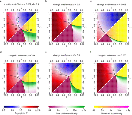
The relevant f − fv parameter space, where fv ≤ f, can be divided into five regions, where the epidemic dynamics follows the distinct patterns exemplified in Figure 2. The area occupied by each region changes depending on the parameter setups, as shown in Figure 3. For example, in the reference setup in Figure 3a (high vaccine effectiveness a = 0.9 and (re-)vaccination rates υ = υr = 0.004, low never-vaccinated fraction d = 0.1 and low immunity waning rate ω = 0.002), the overcritical region (with R* always above 1) occupies the lower left corner. It is enlarged with smaller vaccine effectiveness (a = 0.6, Fig. 3b), larger fraction of the never-vaccinated population (Fig. 3e) and higher waning rate (Fig. 3f), while it shrinks with higher vaccination rate (Fig. 3c). The subcritical region - (with R* always smaller than 1) lies in the opposite corner of the f − fv space, for larger values, and for a fixed fraction of never-vaccinated d tends to decrease for setups where the overcritical region increases. Inside each of the remaining three regions (associated with the +-+, -+, +- scenarios in Figure 2), the specific parameter settings differ by the time to the critical threshold of interest for that region (the last observed switch between subcritical and overcritical epidemic, which for the +-+ region, for example, is the second critical threshold; see Methods for the computation of the times to critical thresholds). For the reference setup (Fig. 3a), the critical threshold is reached after a minimum ∼ 8 months. Decreasing vaccine effectiveness (Fig. 3b), as well as increasing the waning rate (Fig. 3f), enlarges the +-+ region’ and leads to overcriticality sooner, after ∼ 3 and ∼ 4 months respectively, for low fv values. Increasing vaccination rate (Fig. 3c) shrinks the +-+ region. With preferential mixing (Fig. 3d), the +-+ region becomes larger and overcriticality is reached even sooner. Increasing the number of never-vaccinated people (Fig. 3e) shrinks the +-+ region and delays the onset of overcriticality. For all considered parameter setups, except for the one with high (re-)vaccination rate, for all except the +-and the -regions, large asymptotic R* can be expected, which corresponds to short doubling times (Fig. 3).
For various choices of the other parameters, the relevant f − fv parameter space, where fv ≤ f, can be divided into five regions, each associated with a different behavior of the epidemic, exemplified by the five scenarios in Figure 2a. On the diagonal (white dashed line), f = fv, namely the restrictions for VP holders and for the rest of the population are the same. Lower triangles show the time until the last critical threshold: different colour scales correspond to the time until the switch either from a subcritical to an overcritical epidemic (time until overcriticality, violet-green scale), or from an overcritical to a subcritical epidemic (time until subcriticality, yellow-pink scale). Upper triangles show the asymptotic R*, as a function of the values of f and fv (blue-red scale, with blue associated with R* < 1 and red associated with R* > 1). a. Reference setup, with a = 0.9, υ = υr = 0.004, ω = 0.002, d = 0.1 and proportional mixing. The choices of (f, fv) corresponding to the five scenarios exemplified in Figure 2 are denoted by crosses of the same colour. b. Setup with decreased vaccine effectiveness: a = 0.6. c. Setup with increased vaccination rate: υ = υr = 0.008. d. Setup with preferential (instead of proportional) mixing. e. Setup with increased fraction of people who will not get vaccinated: d = 0.3. f. Setup with increased waning rate: ω = 0.005.
These results indicate that VP holders can be granted large freedom, as long as sufficient restrictions are enforced for the rest of the population, to avoid an initially overcritical situation. However, to prevent the epidemic from becoming overcritical after an initial decline in case numbers, restrictions on VP holders need to be timely increased and adapted so that eventually everyone faces the same restrictions. Safe restrictions correspond to the parameters in the sub-critical region, but these are relatively high and could be unacceptable for the population. The -+ and +-+ regions can seem attractive from the aspect of large freedom for the VP holders. Both these regions, however, eventually result in epidemic resurgence and should be avoided. Moving to the +- region with the right timing is a recommendable strategy.
A minimum common restriction level is required to keep the epidemic sub-critical
We compute the minimum common restriction level fmin for the whole population that would be required to avoid an overcritical epidemic in the long-term (Methods):
 where V as is the asymptotic fraction of the immunized in the population
 The resulting values differ depending on the setups of vaccine effectiveness a, revaccination rate υr, the fraction of never-vaccinated population d and immunity waning rate ω (Tab. 1). Even for the most optimistic setup (high a = 0.9, high υr = 0.008, low d = 0.1, low ω = 0.002) we obtain V as = 0.65, and fmin = 0.29. Compared to the current strict restrictions required to contain COVID-19 in some countries, the level of 0.29 restrictions is lower, but it is a considerable reduction of freedom compared to before the pandemic. All remaining realistic parameter setups require high fmin, ranging between 0.46 (for the reference setup) and 0.68 (for the increased d, increased ω as compared to the reference).
Asymptotic level of immunization V as and minimum common restrictions fmin for different parameter setups, for parameters: vaccine effectiveness a, revaccination rate υr, fraction of never-vaccinated d, and waning immunity rate ω. The first row concerns the reference setup; rows below are setups with the same parameters as in the reference setup, but with either one parameter changed (in bold; rows 2–5; same as in Figure 3, apart from preferential mixing, as it is not relevant for common restrictions) or two parameters changed (in bold; rows 6–11).
Discussion
Introducing VPs is widely seen as a means to opening up economies and societies, despite the ongoing epidemic. To inform this discussion, we extend a SIR model to reflect vaccination dynamics and possibly different restrictions for VP holders. A wide range of model parameter choices show the possibility of an epidemic resurgence, even for optimistic parameter setups. The main driver of this phenomenon is the potential lack of immunity of VP holders. With a VP, people enjoy low restrictions while actually being susceptible and potentially contagious because the vaccine was ineffective or the immunity has waned.
VAP-SIRS deliberately keeps several aspects simple (see Methods for model limitations). The advantage of our analysis is the relevance for long-term dynamics, and the focus on avoiding epidemic resurgence. Avoiding another wave is a prudent goal due to threats it poses, in the form of long-term health effects, the deleterious impact on societies and the emergence of new variants.
Our model gives valuable insights into policies pertaining to the introduction of VPs. Model analyses suggest that considerably lowering restrictions for VP holders is only possible when keeping high restrictions on the rest of the population. This situation seems tolerable for the unvaccinated only given high vaccine availability and vaccination speed. The alternative cautious option, i.e. not granting freedoms for VP holders, defeats the purpose of the instrument. Once a large part of the population has been vaccinated, policymakers need to find a new, common restriction level, which could also be achieved through temporary VPs. Our model implies that such common restrictions need to be higher than those initially granted to VP holders, and need to be introduced in time to avoid another wave.
As expected, the model shows that there is a larger selection of admissible restrictions’ setups under high vaccine effectiveness, slowly waning immunity, proportional social mixing, low share of never-vaccinated and higher vaccination rate. At least the latter two parameters are amenable to policy action. Thus, efforts to increase (re-) vaccination speed and encourage people to get vaccinated also extend the margin of lowering restrictions for VP holders as well as eventual common restrictions. Social mixing patterns, such as preferential mixing, can accelerate the infection resurgence in time and, although difficult to change by policymaking, should be monitored. Finally, it is noteworthy that VP holders are less likely to be tested, as they are assumed to be protected and they may exhibit milder symptoms. Therefore, their potential infection is more likely to remain undetected, resulting in an effect similar to that of lowering restrictions. To prevent undesirable outcomes, the testing criteria should not exclude the VP holders. In addition, the VP holders should be widely and regularly tested for antibody level, aiming at detection of such vaccinated that have lost, or have never gained, immunity. Finally, temporary VPs could be considered, with their prolongation conditioned on high antibody level or recent (re-)vaccination.
Data Availability
Not applicable
https://github.com/storaged/VAP-SIRS
Methods
Mathematical model
We introduce a modified susceptible-infectious-recovered-susceptible (SIRS) model [1] (Figure 1a). The population is divided into two subpopulations: those who are not vaccinated (S, I, R) and those who got vaccinated at least once (SV, IV, RV, V). We assume that the group of non-vaccinated susceptible individuals S (and, similarly, infected I and recovered R) is divided into two subgroups: SN and SD. The SN compartment contains such susceptible who will eventually be vaccinated, while those in SD will not. The SD compartment contains not only the subpopulation of children, who are currently not included in the vaccination program, but also those who for health reasons cannot be vaccinated, and finally, individuals who do not vaccinate because of hesitancy.
The SN population is vaccinated with rate υ and effectiveness a. Consequently, the individuals from the SN group populate the vaccinated group V with rate aυ. The individuals in V are considered immune, and we assume that immunization prevents them both from getting infected and infecting others. The SV compartment is composed of S1 and S2 (and, similarly, vaccinated infected IV consists of I1 and I2). Due to vaccine ineffectiveness, people in S1 are perceived as immunized, but in fact are susceptible. S1 is populated from SN with rate (1 − a)υ. The vaccinated from the V group move to the S2 group of susceptibles with immunity waning rate ω. The individuals from the S1 group move to S2 with the same rate ω. The S2 group is the group of vaccinated, but no longer immune, and thus, susceptible individuals. In contrast to S1, we consider that the S2 group is subject to revaccination. Consequently, a fraction of size a of the population from S2 populates V with rate aυr and a fraction of size (1 − a) populates S1 with rate (1 − a)υr. Across the manuscript, we assume υr = υ, but the model is general and different values can be considered. Individuals from S1 move to S2 with rate ω to ensure that the ineffectively vaccinated are revaccinated with the same speed as the ones for which the vaccine was effective.
Some of the susceptibles in S1 (or, similarly, S2) may not get revaccinated fast enough and may become infected and populate I1 (or, I2). Then, as in the classical SIRS model, the I1 (or I2) population recovers and populates group RV with rate γ. We consider that the recovered in RV may also lose the immunity, and become susceptible again and move to S2 with rate κ. We fix κ to 0.002, corresponding to average 500 days duration of natural immunity. There remains uncertainty regarding the waning time for natural immunity, but early evidence indicates it lasts at least 180 days [2, 3, 4]. Hence, we assume an optimistic scenario of natural immunity lasting similarly long as the immunity gained via vaccination. Before the recovered in the RV lose immunity, they might be revaccinated, and, thus, populate the V group with rate υr.
The remaining susceptible subgroups (the SN and SD) may undergo the same classical dynamics, i.e., become infected, recover, and either become susceptible again or, in case of the recovered in the RN subgroup, become vaccinated with rate υ.
Note that for the recovered in the RV or RN groups we assume that vaccination effectiveness is 1, which is substantiated on the basis of the fact that vaccination combined with a previous infection should confer a much stronger protection than only vaccination of a susceptible individual. The following parameters are used to describe population dynamics in the model:
fv, f : restrictions level (for VP holders and others)
β0 : basic transmission rate
βv, β : transmission rate (for VP holders and others)
γ : recovery rate
κ : natural immunity waning rate
a : vaccination effectiveness
υ : vaccination rate
υr : revaccination rate
ω : vaccine-induced immunity waning rate
d : fraction of population that will never get vaccinated
Finally, the following set of ordinary differential equations (ODEs) defines the dynamics
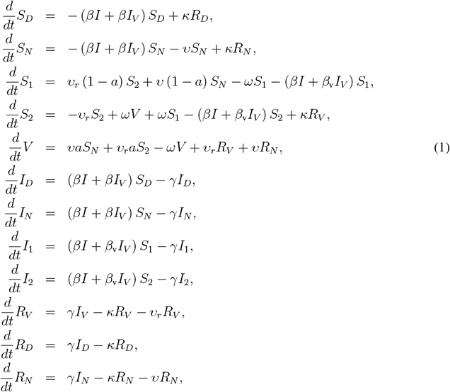 where also the following relations hold
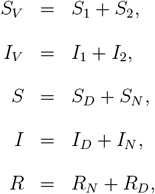 with the constraint S, SV, I, IV, R, RV ≥ 0. Finally, to consider the subpopulation dynamics in terms of fractions of the entire subpopulation, we set
 and denote d to be the fraction of the never-vaccinated population

Modeling restrictions
We assume that the VP holders consist of the following subpopulations of vaccinated at least once: V, SV, IV, RV. Recall that the net effect of all non-pharmaceutical interventions is modeled using parameters fv and f, called restrictions throughout the text. The parameter fv amounts to the level of restriction of contacts, and thus the ability to infect, within the group of VP holders. The parameter f satisfies f ≥ fv and corresponds to restriction of contacts within the rest of the population, as well as between the VP holders and the rest of the population.
The restriction level fv for the VP holders is introduced in the model as a modulator of the transmission rate βv. Specifically, we assume that βv = β0(1 −fv), where β0 is the transmission rate of the SARS-CoV-2 virus without restrictions. We assume fv ranges from 0 to 1, where fv = 0 corresponds to no restrictions enforced on the VP holders, and fv = 1 corresponding to full restrictions. Given that for fv = 0 the reproduction number Rmax = β0/γ = 4, and that the recovery rate γ = 1/6, we obtain the no-restriction transmission rate β0 = 2/3.
Similarly, the transmission rate parameter β = β0(1 − f) describes the transmission rate within the rest of the population and between VP holders and the rest, given the restrictions f.
Proportional versus preferential types of social mixing
The above described model equations are based on the assumption that the social mixing between social groups in the population is proportional to the group sizes (the mass action principle). Instead, preferential mixing can be assumed, where the VP holders are more likely to contact other VP holders, since they have lower restrictions [5]. This preferential bias is proportional to the difference between the restrictions f and fv. To incorporate the preferential mixing effect in the ODE model (Equation 1) we rescale the interaction terms according to the following rules:
 where S + I + R is the non-immune population.
Model simulations
For simulations, we solve the model numerically by means of joint Adams’ and BDF methods, as implemented in the R package deSolve, lsoda method of the ode function [6]. The method monitors data in order to select between non-stiff (Adams’) and stiff (BDF) methods. It uses the non-stiff method initially [7].
To generate the data presented in Figure 1b,c, we use the reference setup of parameters: β0 = 2/3, f = 0.63 (and thus β = 0.247), fv = 0.05 (and thus βv = 0.634), γ = 1/6, κ = 1/500, a = 0.9, υ = υr = 1/250, ω = 1/500, d = 0.1, with initial conditions I = 10−6, ID = d · I = 10−7; IN = (1 − d) · I = 0.9 · 10−6, R = 0, V = 0. Given I(t) resulting from the solution of the model’s ODE system, to present the final results as easier interpretable cases per milion rather than fractions, we re-scale the results by 1M. Additionally, we compute a proxy for the daily incidence number of new cases from the following relation between I (t) and I* (t):
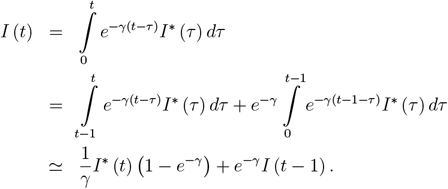 Thus, the I*(t) is computed as
 We proceed similarly to obtain daily incidence numbers
  and for the sum of all infected, and again to make it interpretable in the figures we re-scale it by 1M.
Stability analysis
The vaccination dynamics can be solved explicitly in the absence of infections. Fixing I = IV = R = RV = 0, and assuming υ = υr, we obtain
 For convenience, where it is not needed, we drop the time argument.
Taking an adiabatic approach we linearize the infection dynamics for small I, IV and R under the assumption of slowly varying S, SV and V. In that case, the infection dynamics decouples from the vaccination dynamics and the Jacobian submatrix Jsub for the equations for I and IV is given by:
 Given the Jacobian submatrix, we can approximate the dynamics in a small neighborhood of the I = IV = 0 state as

The instantaneous reproduction number R* and the instantaneous doubling time D
Since the largest and the second largest eigenvalues λmax and λ2 of Jsub are both real, the solution to Equation 3 providing the dynamics of infection numbers of the vaccinated and the rest of the population in time can be written in the following form
 where w1 and w2 are the respective eigenvectors, and c1 and c2 are constants depending on the initial conditions.
Since we have λ2 − λmax ≤ 0, we can approximate the time evolution of infection numbers by
 The largest eigenvalue of Jsub is given by
 whereby it is convenient to express λmax as a function of
  and
and  . We then obtain
 Given the population fractions S(t) and SV (t) at a given time instant t, the linearized dynamics of infections given by Equation 3 has a corresponding two-type Galton-Watson branching process, which is a microscopic description of the dynamics. The two types of the process correspond to the I and IV groups. The type I individuals generate Pois (R1S) offsprings of type I and Pois (R1SV) offsprings of type IV. The type IV individuals generate Pois (R1S) offsprings of type I and Pois (R2SV) offsprings of type IV. The linearized dynamics (3) can then be understood as a mean field limit of the microdynamics described by such a branching process. Moreover, the spectral norm
 of the transition matrix
 of the branching process can be interpreted as the reproduction number of the branching process, since the expected number of infected in generation n grows like const · (R*)n [8]. We refer to R* as the instantaneous reproduction number. The term instantaneous comes from the fact that we are considering the linearized adiabatic dynamics in a small neighborhood of the I = IV = 0 (ref Eq. 3).
The above discrete branching process can be extended to a continuous time branching process by assuming a probability distribution on the generation time, denoted ϕ(γ). The growth of the continuous time branching process const · eαt is characterized by its Malthusian growth parameter, denoted α. The relation between the instantaneous reproduction number R*, the distribution φ (τ) and the Malthusian parameter α for such a branching process is given by
 where ℒφ (α) is the Laplace transform
  of the distribution φ [8]. Since the setting of ODE model (1) implies exponential distribution of the generation time, i.e, φ(γ) = Exp (γ), the following relation holds: α = γ (R* − 1).
By Equation 5, the Malthusian parameter α for our dynamics is given by the largest eigenvalue λmax. Hence we obtain the relation between the instantaneous reproduction R* and the λmax as λmax = γ (R* − 1). Note that since both S and SV are functions of time, so are λmax and R*.
It is noteworthy that in the above equations, all R1, R2, R1S and R2SV, and R* should be seen as reproduction numbers, but of a different nature [9]. R1 and R2 are reproduction numbers taking into account the restrictions f and fv, respectively. The R1S and R2SV are also group specific, but in addition incorporate the respective group sizes. Finally, R* combines all these factors together.
Having this and Equation 5, we define the instantaneous doubling time at time, denoted t D(t), as the solution D of eγ(R*(t)−1)·D = 2. Such obtained doubling times are featured in Figure 2b.
The times of transitions between subcritical and overcritical epidemics
The analysis of the linearized dynamics around I = IV = 0 allows us to determine transitions between subcritical and overcritical epidemics. Such transitions occur at the time instants t at which λmax(t) = 0, or, equivalently, at R*(t) = 1. We thus find that for given values of S(t) and SV (t) the critical times t for transitions between subcritical and overcritical epidemics are the roots of the equation
 The obtained critical threshold times are plotted in the lower triangles of the panels in Figure 3 in the main text. In the case of proportional mixing the above equation is equivalent to:

Asymptotic structure of the population
The asymptotic structure of the population in terms of the sizes of the subpopulations V, SV and SD can be easily obtained by setting I = IV = R = RV = 0 and computing the stable stationary solution for V as, Sas and  of our ODE system (1):
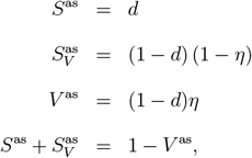 where
where
 can be seen as the actual immunization rate in the population, and is expressed as a function of vaccine effectiveness a and the ratio of the immunity waning rate ω and the revaccination rate υr. The obtained values correspond to the structure in the limit t → ∞ and represent the structure to which the population converges in the long term.
Having this, we obtain the asymptotic instantaneous reproduction number R* by inserting the asymptotic values Sas and  into Equation 8. These values are plotted in the upper triangles in the panels of Figure 3 in the main text.
Finally, we solve for such minimum common restrictions f = fv = fmin, which will result in instantaneous reproduction number R* = 1 for the different vaccine effectiveness and vaccination rate setups. Hence fmin is found from  as
as

Model limitations
VAP-SIRS is not compartmentalized for age groups and does not consider deaths or healthcare system limitations like some other models, albeit in the context of exploring different parameters than larger freedom for VP holders [10, 11, 12, 13, 14, 15]. Deaths could be taken into account through a straightforward modification of the model, which would however lead to more parameters. In this case, the fact that vaccination reduces the risk of death would have to be accounted for. The impact of deaths on public health and society, which is very important especially when the epidemic becomes overcritical, can be indirectly assessed based on the number of infection cases. In general, features such as age groups and deaths, however, do not add further insights into the questions which are the focus of our study, namely, the long-term effects of VPs and avoiding overcritical dynamics. In this context, the advantage of our model is that it is enriched in features such as revaccinations and waning immunity, which are particularly relevant in the long term.
Nevertheless, possible extensions to our model could include inter-individual or age-dependent variations in immunity, which is also relevant for people with severe chronic conditions or immunodeficiencies, or changes in behaviour over time. The presented analysis has been performed assuming that without restrictions, the maximum reproduction number of the virus is Rmax = 4. More transmittable variants could easily be modeled by fixing higher values of Rmax. Similarly, our results do not account for the possibility of immune escape variants, but such variants could be considered using our model by fixing smaller vaccine effectiveness than the values we considered. Asymptotic endemic states of the ODE system (1) could easily be computed, but are not discussed here due to space constraints. Finally, another limitation of our analysis is that not all parameter values are exactly known, such as the post-vaccination or natural immunity waning time. We, however, fix optimistic values for such parameters, and show that unfavorable infection dynamics can still be obtained even under optimistic assumptions.
Data Availability
Not applicable
Code Availability
The VAP-SIRS model was implemented using R version 4.0.2 along with the shiny package to build an interactive web application that allows to simulate the model. The code of the model is available online in the GitHub repository: https://github.com/storaged/VAP-SIRS, and the on-line tool is available http://bioputer.mimuw.edu.pl:85/VAP-SIRS/. The code to generate Fig 2 and Fig 3 from the main text is available at https://github.com/eMaerthin/Fig2_Fig3.
End notes
Author contributions
AG, KG, TK, and ES conceived the VAP-SIRS model - with input and feedback on the model and results from TC, GG, MP, EP and MR. TK performed the stability analysis. KG implemented model simulations and the Shiny application for visualizations. MB implemented the stability analysis. SC, TC, EP, and MR performed literature search. ES supervised the study. All authors wrote and provided critical feedback to the manuscript.
Competing interests
Other projects in the research lab of ES are co-funded by Merck Healthcare KGaA.
Additional information
Correspondence and requests for materials should be addressed to ES. Reprints and permissions information is available at www.nature.com/reprints.
Acknowledgements
SC acknowledges support by University of Malta. TC has received funding from the European Union’s Horizon 2020 research and innovation programme under grant agreement No 101016233 (PERISCOPE) GG acknowledges support by the University of Trento within the COVID-19 Strategic Project MOSES (Models for Reasoning about the Spreading of Diseases). MP was supported by the Slovenian Research Agency (Grant Nos. P1-0403 and J1-2457). EP acknowledges support by the University of Crete. ES acknowledges funding by the Polish National Science Centre OPUS grant no 2019/33/B/NZ2/00956 and SONATA-BIS grant no 2020/38/E/NZ2/00305.
Footnotes
↵* Shared first authorship


