
ABSTRACT
Laboratory experiments have revealed the meteorological sensitivity of the virus of the coronavirus disease 2019 (COVID-19). However, no consensus has been reached about how the meteorological conditions modulate the virus transmission as it is constrained more often by non-meteorological factors. Here, we find that the non-meteorological factors constrain statistically-least the growth rate of cumulative confirmed cases in a country when the cases arrive around 2500-3000. The least-constrained growth rate correlates with the near-surface ultraviolet flux and temperature significantly (correlation coefficients r=−0.55±0.08 and −0.45±0.08 at p < 10−5, respectively). In response to increases of 1W/m2 ultraviolet and 1°C temperature, the growth rate decreases by 0.33±0.11% and 0.18±0.08% per day, respectively. The response to the ultraviolet flux exhibits a delay by about 7 days, providing an independent measure of the incubation period. Our quantifications imply a seasonality of COVID-19 and a high risk of a pandemic resurgence in the upcoming boreal winter, suggesting a need for seasonal adaption in public policies.
Introduction
It has attracted extensive attention whether the coronavirus disease 2019 (COVID-19) will spread more in the coming winter. Winters are often accompanied by peaks of virus transmissions, such as some Human coronaviruses1 and influenza2. These seasonalities are typically explained in terms of modulations of meteorological conditions on the virus survival, e.g.,3. This knowledge has raised fears that COVID-19 may surge when the seasons change.
A way to predict the COVID-19 transmissions in the winter is to investigate the responses of the virus survival and transmission to the winter weather conditions. Laboratory experiments revealed that the ultraviolet radiation and air temperature modulates the airborne survival of the virus strongly4–6. Several studies have attempted to extract epidemiological evidence, e.g.,7–10, through studying the correlations between the number of infections or mortality and the corresponding meteorological conditions using data from priorly selected cities. Their conclusions, however, are controversial. Some attempts did not find the correlation, e.g.,6,7, whereas the others reported weak or moderate correlations, e.g.,8–10. The results are not conclusive, mainly because the meteorological modulations are constrained by non-meteorological effects. In the current work, we identify the least-constrained growth rate of the infection and quantify its response to meteorological conditions statistically.
Results
An uncontrolled outbreak of COVID-19, e.g.,11, starts with an exponential growth, the rate of which is presumably modulated by external factors such as weather4–6. We estimate the growth rate through a sliding window regression for each country and investigate its response to meteorological conditions across all countries, in contrast to the above-mentioned works7–10, which analyzed the number of confirmed cases or mortality from prior selected cities directly. Therefore, our results allow capturing straightforward the modulation of the weather and are not subject to potential statistical bias.
The least-constrained growth rate
Ideally, outbreaks of infectious diseases e.g.,11–13, are typically characterized by two phases with the uncontrolled first phase showing stable exponential growth followed by a second phase with a decreasing growth rate usually after effective artificial controllers14,15 (as sketched by the green lines in Figures S1b and S2a). The realistic evolution of the regressed growth rate of confirmed cases decreases largely with time, which can be divided into three primary stages (Figure S1 as an example and Figure S2 for all countries). In the beginning, infections cannot be confirmed timely and can accumulate until sufficient tests, which is different from the uncontrolled ideal model. Therefore, in Phase I, the decreasing growth rate reflects more the improvement of the capability than the infection growth. In Phase III, the decreasing growth rate could be explained as responses to artificial interventions or controllers, e.g., travel restrictions and changes in human behaviors, e.g.,16,17. Also, at the late stage, cured cases are not infectious anymore and therefore lower the growth rate. Phase III corresponds to the decline stage of the ideal evolution model.
Therefore, it is most likely in Phase II, in-between the Phases I and III, where the uncontrolled transmission of COVID-19 is recorded timely and sufficiently. Phase II is characterized by a relatively stable growth rate (Figures S1b and S2a), reflecting presumably the most modulation from the weather. In practical, instead of delimiting definitely the stage II for each country, we determine the most stage-II-representative growth rate, referred hereafter as least-constrained growth rate, for all countries through a single-parameter optimization (see “Methods”). The optimization maximizes the correlation between the least-constrained growth rate and meteorological variables. We obtain the solution of the optimization when the accumulative confirmed cases arrive statistically around 2500-3000 (in Phase II in Figure S2a).
Impact of meteorological factors on the growth rate
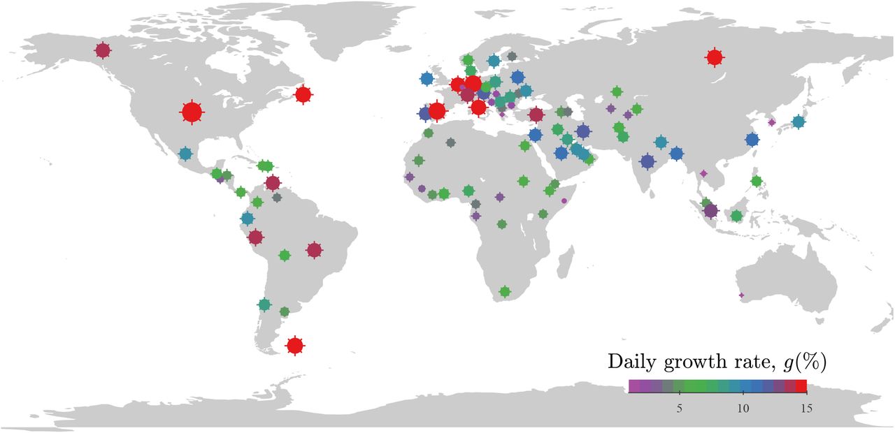
In Figure 1, Africa, central Asia and Central America are generally associated with low least-constrained growth rates, whereas high growth rates are observed in middle and high latitudes of North America and Europe. The obvious spatial clusters of the growth rate suggest its potential links to meteorological conditions. The growth rate exhibits significant correlation with the ultraviolet (UV) flux and the air temperature (r=−0.55±0.08 and −0.45±0.08 at p <<0.01, in Figures 2a and 2b, respectively), but not with the other meteorological conditions, namely, wind speed, relative humidity, diurnal temperature range, and precipitation (p >=0.05, Figures 2c-2f). The regressions (in red in Figures 2a and 2b) quantify the responses. An increase in UV flux by 1 W/m2 is associated with a decrease in the growth rate by 0.33±0.11% per day, and an increase of the temperature by 1°C is associated with a decrease in the growth rate by 0.18±0.08% per day.

Global distribution of the daily growth rate g of COVID-19 cases. Each point represents one country/region. Both the color and the size of the symbols represent the growth rate. The growth rate is estimated through a sliding window regression and optimization detailed in “Methods”.

Correlation between the daily growth rate g and six meteorological variables, (a) the ultraviolet (UV) the flux in the range 250-440nm, (b) the air temperature at 2m above the surface, (c) the diurnal temperature range, (d) the relative humidity, (e) the wind speed at the height of 10m, and (f) the precipitation. In each panel, one cross represents one country, corresponding to one red cross displayed in Figure S2a; the solid red line presents a robust regression to a linear model g = β1 * x + β0 through the least absolute deviations method, and the dashed and dotted lines display the significance level α = 0.05 and 0.01, respectively. Here, x denotes one of the above six variables, and β1 and β0 denote the parameters to be determined. The regression results are displayed in red on the bottom of each panel, while the Pearson correlation coefficient r is printed on the upright conner, in the format of r ± Δr[rl, ru]. Here, r and Δr are the mean coefficient and its standard deviation estimated through a bootstrapping method, and rl and ru are the lower and upper bounds for a 95% confidence interval. Also displayed on the top is the p-value for testing the hypothesis of no correlation.
A measure of the incubation period
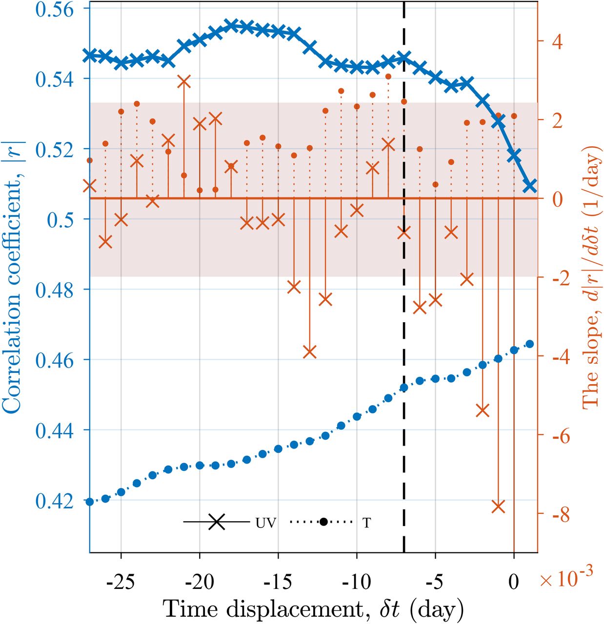
Note that the above correlation and regression analyses involve a time displacement of 7 days between the meteorological variables and the growth rate. The correlation between the growth rate and the UV flux (but not the temperature) weakens suddenly as the time displacement decreases when the displacement is shorter than 7 days (Figures 3). The displacement indicates the presence of an incubation period as revealed previously18,19. The clinical study19 suggests that the incubation does not follow a normal distribution but is characterized by a positive skew (more cases occurred below the mean) with a median of 5.1 days and a mean of 6.4 days, whereas a cross-sectional and forward follow-up analysis18 reported a median incubation of 7.76 days. The discrepancy might be due to sampling bias in the forward follow-up approach which is less capable of detecting incubations shorter than four days. Similarly to the forward follow-up approach, our sliding window in the cross-correlation approach (Figure 3) captures the cases with incubation periods over the most frequency value, and therefore our diagnosis is consistent more with the forward follow-up analysis. Our results provide independent evidence of the incubation period by correlations from all countries, using approaches completely different from the existing estimations.

The absolute correlation coefficients |r| of the growth rate with the UV flux and temperature T, as functions of the time displacement δt := tUV,T − τ, and their slopes calculated using the centered differencing method. Here, tUV,T is the center of the sampling window of UV or T, whereas τ is the center of the sliding window in which the growth rate is regressed, as instanced in Figure S1. The shadow illustrates one standard deviation of the slopes below and above the average slop. At δt<-7 as displayed by the black line, the slope of rUV is below the shadow, which is attributable to the incubation period of COVID-19.
Discussion
In “Results”, we illustrate that the least-constrained growth rate exhibits obvious spatial clusters and significant correlation with the meteorological conditions, namely, UV flux and temperature. The UV correlation exhibits a delay of about seven days, at the temporal scale of the incubation period. While the spatial clusters and the correlation might be attributed to the spatial difference of socioeconomic factors20,21, the delay cannot. The variations of socioeconomic factors are overall at temporal scales much longer than that of the delay, which can neither modulate the COVID-19 nor respond to the UV flux at the time scale of the incubation period.
To explain the correlation, in the current section, we explore potential causalities between the UV flux and the growth rate.There are at least three factors through which meteorological conditions can modulate the transmission. The first is human behaviors. When the temperature is low, humans typically spend more time indoors, with reduced social distancing and less ventilation than outdoors. As an example, schools are places of enhanced influenza transmission22 for intense indoor activities. The second factor is the immune system of susceptible hosts. Solar radiation drives changes in the human immune system by modulating melatonin23 and/or vitamin D24–26.
The last but might be the most important factor is the survival of the virus, namely the virucidal effect of UV. Evidence has revealed that the aerosols as a medium of transmission of COVID-19, as the virus remains active on the surfaces for several hours to days14. Intense solar radiation may inactivate the virus on the surface through the physical properties (i.e., shape, size) and the genetic material of the virus5,27,28. Simulation results suggested that 90% of the virus can be inactive under summer daytime for 6 minutes, whereas the virus becomes inactive for 125 minutes under night condition4. In addition, high temperature shortens the virus survival6,29,30. On the opposite, low temperature is in favor of prolonging survival on infected surfaces and aerosols, which promotes the diffusion of the infection. The modulation of relative humidity, on the other hand, is negligible, as supported by laboratory experiments4, which is different from the sensitive modulation on the influenza virus survival3 and transmission31.
The 7-day-delayed response to the UV flux (Figure 3) reflects the incubation period, whereas the response to the temperature does not exhibit a delay. A potential scenario is that temperature variation is characterized by a temporal scale longer than the incubation period, and therefore cannot resolve the incubation period. Another potential scenario is that the temperature might not be an independent driver of the transmission but a response to solar radiation. The temperature correlates significantly with the UV flux (r=0.78±0.05 at p=5.8×10⁻²²). We carried out a canonical-correlation analysis, e.g.,32, between the growth rate and the UV flux and temperature, resulting in a canonical correlation coefficient cUV,T =−0.56±0.08. The canonical correlation coefficient is close to the correlation of UV rUV =−0.55± 0.08 (Figure 2a), which implicates that using both the UV and temperature as predictors can not explain more variance of the growth rate than using the UV alone.
The dominant impact of the UV flux can drive a seasonality of COVID-19 transmission and explain the following geographic dependence of COVID-19. (1) The mortality exhibits a latitudinal dependence26. (2) The late outbreak in Africa and arid central Asia is attributable to intense UV flux due to the low cloud fraction prior. (3) The onset of the Asian summer monsoon, increases clouds in early May33 and yields low UV flux, which may account for the late outbreak in India and many southeastern Asia countries until early May. (4) The decrease in UV and temperature during the coming austral winter can contribute to the sharp increase in South America. For example, both the confirmed and dead cases in Brazil ranked second in the world since 13 June.
The current study provides epidemiological support for the hypothesis that the ultraviolet radiation and air temperature drives the COVID-19 transmission26. Our results also implicate a seasonality of COVID-19 and provide an independent measure of the incubation period. The virus transmits more readily during winter and during the season of global monsoon, which impacts about 70% of the global population34. Accordingly, we predict a high possibility of a resurgence in the next boreal winter and suggest to adapt the public policy according to the seasonal variability.
Methods: Daily growth rate of COVID-19 cases
The current section extracts a daily infection growth rate for each country from the data of confirmed cases, through a sliding window regression, optimization, cross-correlation, and unit conversion.
A sliding window regression for describing the evolution of the outbreak
The early stage of an uncontrolled outbreak is characterized by an exponential growth with time, e.g.11,14. As an example, Figure S1a displays the cumulative confirmed case number y(t) as a function of time t, which follows the exponential law largely. Therefore, we fit the y(t) to an exponential model y = aeb(t−τ) in a 28day-wide sliding window. (Note that the conclusions of the current work are qualitatively not subject to the window size here, learn from the same analyses but with different window sizes from 16 to 60 days, which are not displayed here.) Here, τ denotes the center of the sliding window, a measures the confirmed cases at τ, and the exponent factor b measures the growth rate. Measuring the goodness of the regression is r2, which is equal to the square of the correlation coefficient between y(t) and its regression value. A low r2 represents the growth does not follow the exponential law well. We repeat the regression at τ= 2, 4, …, 170 days yielding a and b as functions of τ. Displayed in Figure S1b is b(τ) for Afghanistan as an example.
Implementing the sliding window regression for all countries results in a(τ), b(τ), and r2(τ) for all countries. Scattered in Figures S2a and S2b, are a(τ) and r2(τ) against b(τ) for all countries, respectively. We exclude the b values associated with r2 <0.9. At r2 <0.9, b exhibits a dependence on r2, which could be explained in terms of the three Phases (in “Results”). In Phase III and as a response to the artificial controllers, the growth stagnates and does not follow the exponential law anymore.
An optimization for extracting the least-constrained growth rate
In principle, all the regressed growth rates b values from all countries could be used for correlation analyses. However, for a given country, the regressed b values are not completely independent of each other due to the overlapped sampling associated with our sliding window. Therefore, in the current subsection, we select only one regressed growth rate, denoted as bm, for each country. We select bm as the maximum b at a> θa where θa is a threshold value. θa is optimized by maximizing the absolute correlation coefficient |r(θa)| between bm(θa) and the corresponding meteorological parameters. The coefficients for the UV flux and temperature |rUV (θa) | and |rT (θa)| are displayed in Figure S3 as functions of θa. |rUV (θa)|, greater than |rT (θa)|, maximizes at θa=2500. The red crosses in Figure S2a denote bm at θa = 2500, namely, the maximum b at a >2500. Most of these crosses are between 2500< a <3000, suggesting the growth is modulated statistically strongest by the meteorological conditions when there are about 2500-3000 confirmed cases. As an example, the red symbols in Figure S1 illustrate the determined bm and the associated time window.
A cross-correlation for diagnosing the incubation period
Note that the correlation analyses above are implemented with a time displacement between the sampling window of the growth rate and that of the meteorological variables δt := tUV,T − τ, to avoid the contamination from the COVID-19 incubation period, e.g.,18. We diagnosis the incubation period through cross-correlation analyses.
We first calculate the absolute correlation coefficient |rUV| between 28d-averaged UV flux and bm as a function of the displacement δt. The resultant |rUV (δt)| is displayed as the solid blue line in Figure 3. The slope of the blue line d |rUV|/dδt is denoted as the red crosses. At −7d< δt <0, the slope d |rUV|/dδt is beyond its standard deviation (outside the shadow), reflecting the correlation decrease sharply as the δt increases. We attribute this sharp decrease to the overlapping of the incubation period with the 28d-wide UV simpling window. Note that the identification of the incubation period is not subjective to the threshold θa, which is learned from the same analyses but with different θa =103.1, 103.2, …, 103.8 (not displayed here).
The dotted line and bars display the correlation between bm and temperature, and its slope, which does not exhibit a similar sudden drop.
Conversing the growth rate into percentage
According to our regression model, bm is an exponent and  measures the ratio of the regressed number of confirmed cases of one day over that of the previous day. Therefore,
  is the daily growth rate by percentage. When bm ≈0, bm is already a first-order approximation of g due to
  , since eb can be expanded into Taylor polynomial
  . Here, 𝒪(b2) denotes a variable with absolute value at most some constant times |b2| when b is close enough to 0. In “Results”, the analyses are based on g.
Acknowledgments
This study was funded by the National Science Foundation of China (41888101, 41822101 and 41971022), Deutsche Forschungsgemeinschaft (DFG HE6915/1-1), Strategic Priority Research Program of the Chinese Academy of Sciences (XDB26020000), the State Administration of Foreign Experts Affairs of China (GS20190157002), fellowship for the National Youth Talent Support Program of China (Ten Thousand People Plan). Support from the Swedish Formas (Future Research Leaders) project is also acknowledged. We used the COVID-19 data of cumulative confirmed cases until 20 July of 2020 at a country level from COVID-19 Data Repository by the Center for Systems Science and Engineering (CSSE) at Johns Hopkins University. The daily meteorological variables are extracted from the ERA5 reanalysis dataset from the European Centre for Medium-Range Weather Forecasts (ECMWF) (C3S, 2017). The meteorological variables analyzed herein include the air temperature at 2m above the surface (land, sea or inland waters), precipitation, relative humidity, wind speed at the height of 10m, downward UV radiation flux at the surface (UV, in the range 250-440 nm), and diurnal temperature range. The daily mean meteorological data were averaged for each country to compare with the country-level COVID-19 data.
References


