Abstract
As severe acute respiratory syndrome coronavirus 2 (SARS-CoV-2) spreads, the susceptible subpopulation declines causing the rate at which new infections occur to slow down. Variation in individual susceptibility or exposure to infection exacerbates this effect. Individuals that are more susceptible or more exposed tend to be infected and removed from the susceptible subpopulation earlier. This selective depletion of susceptibles intensifies the deceleration in incidence. Eventually, susceptible numbers become low enough to prevent epidemic growth or, in other words, the herd immunity threshold is reached. Here we fit epidemiological models with inbuilt distributions of susceptibility or exposure to SARS-CoV-2 outbreaks to estimate basic reproduction numbers (R0) alongside coefficients of individual variation (CV) and the effects of containment strategies. Herd immunity thresholds are then calculated as 1 − (1/R0)1/(1+CV2) or 1 − (1/R0)1/(1+2CV2), depending on whether variation is on susceptibility or exposure. Our inferences result in herd immunity thresholds around 10-20%, considerably lower than the minimum coverage needed to interrupt transmission by random vaccination, which for R0 higher than 2.5 is estimated above 60%. We emphasize that the classical formula, 1 − 1/R0, remains applicable to describe herd immunity thresholds for random vaccination, but not for immunity induced by infection which is naturally selective. These findings have profound consequences for the governance of the current pandemic given that some populations may be close to achieving herd immunity despite being under more or less strict social distancing measures.
Scientists throughout the world have engaged with governments, health agencies, and with each other, to address the ongoing pandemic of coronavirus disease (COVID-19). Mathematical models have been central to important decisions concerning contact tracing, quarantine, and social distancing, to mitigate or suppress the initial pandemic spread1. Successful suppression, however, may leave populations at risk to resurgent waves due to insufficient acquisition of immunity. Models have thus also addressed longer term SARS-CoV-2 transmission scenarios and the requirements for continued adequate response2. This is especially timely as countries apply, relax and reapply lockdown measures with varying levels of success in tackling national outbreaks.
Here we demonstrate that individual variation in susceptibility or exposure (connectivity) accelerates the acquisition of immunity in populations. More susceptible and more connected individuals have a higher propensity to be infected and thus are likely to become immune earlier. Due to this selective immunization by natural infection, heterogeneous populations require less infections to cross their herd immunity threshold (HIT) than suggested by models that do not fully account for variation. We integrate continuous distributions of susceptibility or connectivity in otherwise basic epidemic models for COVID-19 which account for realistic intervention effects and show that as coefficients of variation (CV) increase from 0 to 5, HIT declines from over 60%3,4 to less than 10%. We then fit these models to series of daily new cases to estimate CV alongside basic reproduction numbers (R0) and derive the corresponding HITs.
Effects of individual variation on SARS-CoV-2 transmission
SARS-CoV-2 is transmitted primarily by respiratory droplets and modelled as a susceptible-exposed-infectious-recovered (SEIR) process.
Variation in susceptibility to infection
Individual variation in susceptibility is integrated as a continuously distributed factor that multiplies the force of infection upon individuals5 as


 where S(x) is the number of individuals with susceptibility x, E(x) and I(x) are the numbers of individuals who originally had susceptibility x and became exposed and infectious, while R(x) counts those who have recovered and have their susceptibility reduced to a reinfection factor σ due to acquired immunity. δ is the rate of progression from exposed to infectious, γ is the rate of recovery or death, Φ is the proportion of individuals who die as a result of infection and λ(x) = (β/N) ∫[ρE(y) + I(y)] dy is the average force of infection upon susceptible individuals in a population of size N and transmission coefficient β. Standardizing so that susceptibility distributions have mean ∫ xg(x) dx = 1, given a probability density function g(x), the basic reproduction number is
 where ρ is a factor measuring the infectivity of individuals in compartment E in relation to those in I. The coefficient of variation in individual susceptibility
  is explored as a parameter. Non-pharmaceutical interventions (NPIs) designed to control transmission typically reduce β and hence R0. We denote the resulting controlled reproduction number by Rc The effective reproduction number Reff is another useful indicator obtained by multiplying R, by the susceptibility of the population, in this case written as Reff(t) =Rc(t) ∫ xS(x, t) dx/N(t) to emphasize its time dependence.
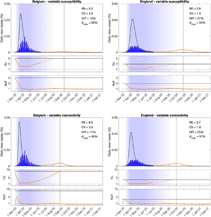
Top panels of Figure 1 depict model trajectories fitted to suppressed epidemics (orange) in 2 European countries (Belgium and England) assuming gamma distributed susceptibility and no reinfection (σ = 0). We estimate: R0 rounding 5 (Belgium) and 2.9 (England); individual susceptibility CV reaching 3.9 (Belgium) and 1.5 (England); and overall intervention efficacy at maximum (typically during lockdown) being 60% (Belgium) and 54% (England). Other estimated parameters are the day when NPIs begin to affect transmission, after which we assume a linear intensification from baseline over 21 days, remaining at maximum intensity for Tmax days and linearly lifting back to baseline over a period of Tllift days (both Tmax and Tllift are estimated). Denoting by d(t) the proportional reduction in average risk of infection due to interventions, in this case we obtain Rc(t) = [1 − d(t)]R0 which is depicted for each country, alongside Reff(t), underneath the respective epidemic trajectories. To assess the potential for case numbers to overshoot if NPIs had not been applied, we rerun the model with d(t) = 0 and obtain the unmitigated epidemics (black). Further details are described in Methods.
Variation in susceptibility (top panels); variation in connectivity (CV reducing in proportion to social distancing) (bottom panels). Susceptibility or connectivity factors implemented as gamma distributions. Suppressed wave and subsequent dynamics in Belgium and England (orange). Estimated epidemic in the absence of interventions revealing overshoot (black). Blue bars are daily new cases. Controlled (Rc) and effective (Reff) reproduction numbers are displayed on shallow panels underneath the main plots. Blue shades represent social distancing (intensity reflected in Rc trends and shade density). Rc values in the dotted portion of the orange lines do not interfere with the fittings and are only used to illustrate how the epidemic may unfold beyond the data analysed here. Consensus parameter values (Methods): δ = 1/4 per day; γ = 1/4 per day; and ρ = 0.5. Fraction of infected individuals identified as positive (reporting fraction): 0.06 (Belgium); 0.024 (England). Basic reproduction number, coefficients of variation and social distancing parameters estimated by Bayesian inference as described in Methods (estimates in Extended Data Tables 1 and 3). Curves represent mean model predictions from 104 posterior samples. Orange shades represent 95% credible intervals. Vertical lines represent the expected time when herd immunity threshold will be achieved.
Estimates generated from model fit to the national datasets are in the grey shaded rows. The remaining rows provide the region-specific estimates. Best parameter estimates are presented as a bold median bounded by the lower and upper ends for the 95% credible interval. Model runs are initiated on the day (t0) when reported cases surpassed 1 in 5 million individuals: Belgium (day 1); England (day 29); Portugal (day 3); Spain (day 8).
Estimates generated from model fit to the national datasets are in the grey shaded rows. The remaining rows provide the region-specific estimates. Best parameter estimates are presented as a bold median bounded by the lower and upper ends for the 95% credible interval. Model runs are initiated on the day (t0) when reported cases surpassed 1 in 5 million individuals: Belgium (day 1); England (day 29); Portugal (day 3); Spain (day 8).
Estimates generated from model fit to the national datasets are in the grey shaded rows. The remaining rows provide the region-specific estimates. Best parameter estimates are presented as a bold median bounded by the lower and upper ends for the 95% credible interval. Model runs are initiated on the day (t0) when reported cases surpassed 1 in 5 million individuals: Belgium (day 1); England (day 29); Portugal (day 3); Spain (day 8).
Variation in connectivity
In a directly transmitted infectious disease, such as COVID-19, variation in exposure to infection is primarily governed by patterns of connectivity among individuals. We incorporate this in the system (Equations 1-4) assuming that individuals mix at random (but see Methods for more general formulations that enable other mixing patterns). Under random mixing and heterogeneous connectivity6, the force of infection is written as λ(x) = (β/N)(∫ y[ρE(y) + I(y)] dy/∫ yg(y) dy), the basic reproduction number is
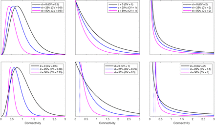
 Rc(t) is as above and Reff(t) is derived by a more general expression given in Methods. The results from this basic variable connectivity model are shown in Extended Data Figure 1). To allow for the possibility that social distancing (d) may change not only the scale but also the shape of connectivity distributions, we consider an extended model where connectivity is reformulated as (1 − d)[1 + (1 − d)(x − 1)] (Extended Data Figure 2). This does not change the way the model is written but special care is needed in analysis and interpretation to account for the dynamic contact patterns. The basic reproduction number, in particular, depends explicitly on a CV which is now dependent on social distancing.
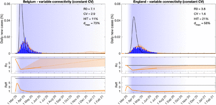
Variation in connectivity (constant CV). Connectivity factors implemented as gamma distributions. Suppressed wave and subsequent dynamics in Belgium and England (orange). Estimated epidemic in the absence of interventions revealing overshoot (black). Blue bars are daily new cases. Controlled (Rc) and effective (Reff) reproduction numbers are displayed on shallow panels underneath the main plots. Blue shades represent social distancing (intensity reflected in Rc trends and shade density). Rc values in the dotted portion of the orange lines do not interfere with the fittings and are only used to illustrate how the epidemic may unfold beyond the data analysed here. Consensus parameter values (Methods): δ = 1/4 per day; γ = 1/4 per day; and ρ = 0.5. Fraction of infected individuals identified as positive (reporting fraction): 0.06 (Belgium); 0.024 (England). Basic reproduction number, coefficients of variation and social distancing parameters estimated by Bayesian inference as described in Methods (estimates in Extended Data Table 2). Curves represent mean model predictions from 104 posterior samples. Orange shades represent 95% credible intervals. Vertical lines represent the expected time when herd immunity threshold will be achieved.
Individual variation in connectivity is originally implemented as a gamma distribution of mean 1 parameterised by the coefficient of variation (CV) (black). Social distancing is initially implemented as a reduction in connectivity by the same factor to every individual, from x to (1 − d)x (top panels). A more general formulation where CV may reduce with social distancing is implemented by modifying x to (1 − d)[1 + (1 − d)(x − 1)] (bottom panels).
Applying this model to the same epidemics as before we obtain the bottom panels of Figure 1. The estimated epidemiological parameters are: R0 rounding 8.9 (Belgium) and 3.7 (England); individual connectivity CV reaching 3.9 (Belgium) and 1.6 (England); and intervention efficacy during lockdown being 45% (Belgium) and 37% (England). The reported CVs correspond to baseline contact patterns.
Comparing the two models, variation in connectivity systematically leads to higher R0 estimates. The effect attributed to NPIs is lower in England than in Belgium. In both countries, contacts appear to reach minimal levels around lockdown in April (Rc plots), beginning to re-intensify thereafter but remaining below about half of pre-lockdown levels by the end of the data series used for model fittings (solid portions of the Rc line), consistently with the CoMix contact survey7. To illustrate how the epidemic may unfold beyond the data used in this study we simulate a hypothetical scenario whereby contacts continue to reactivate linearly until eventually reaching the pre-pandemic baseline. This leads to low epidemic activity over a period that coincides with the Summer months, followed by a resurge as contacts intensify. This resurgence is likely to be aggravated by seasonality as the Winter approaches, although seasonality has not been included in our models. The percentage of the population required to be immune to curb the epidemic and prevent future waves when interventions are lifted appears remarkably conserved across models: 10 vs 11% (Belgium); and 27 vs 25% (England).
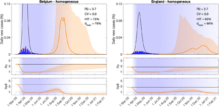
We then fit to the same data the model constrained by CV = 0, i.e. assuming no relevant heterogeneity in susceptibility or exposure to infection. The results are shown in Figure 2. In this case epidemic potential is considerably larger and hence the effect attributed to NPIs to fit the data must also be larger. The percentage of the population required to be immune to prevent epidemic growth when interventions are lifted rises to 73% (Belgium) and 63% (England).
Suppressed wave and subsequent dynamics in Belgium and England (orange). Estimated epidemic in the absence of interventions revealing overshoot (black). Blue bars are daily new cases. Controlled (Rc) and effective (Reff) reproduction numbers are displayed on shallow panels underneath the main plots. Blue shades represent social distancing (intensity reflected in Rc trends and shade density). Rc values in the dotted portion of the orange lines do not interfere with the fittings and are only used to illustrate how the epidemic may unfold beyond the data analysed here. Consensus parameter values (Methods): δ = 1/4 per day; γ = 1/4 per day; and ρ = 0.5. Fraction of infected individuals identified as positive (reporting fraction): 0.06 (Belgium); 0.024 (England); 0.09 (Portugal); 0.06 (Spain). Basic reproduction number, coefficients of variation and social distancing parameters estimated by Bayesian inference as described in Methods (estimates in Extended Data Table 4). Curves represent mean model predictions from 104 posterior samples. Orange shades represent 95% credible intervals.
Estimates generated from model fit to the national datasets are in the grey shaded rows. The remaining rows provide the region-specific estimates. Best parameter estimates are presented as a bold median bounded by the lower and upper ends for the 95% credible interval. Model runs are initiated on the day (t0) when reported cases surpassed 1 in 5 million individuals: Belgium (day 1); England (day 29); Portugal (day 3); Spain (day 8).
Herd immunity thresholds
Individual variation in risk of acquiring infection is under selection by the force of infection, whether individual differences are due to biological susceptibility, exposure, or both. The most susceptible or exposed individuals are selectively removed from the susceptible pool as they become infected and eventually recover (some die), resulting in decelerated epidemic growth and accelerated induction of immunity in the population. In essence, the herd immunity threshold defines the percentage of the population that needs to be immune to reverse epidemic growth and prevent future waves. When individual susceptibility or connectivity is gamma-distributed and mixing is random, HIT curves can be derived analytically8 from the model systems (Equations 1-4, with the respective forces of infections). In the case of variation in susceptibility to infection we obtain
 while variable connectivity results in
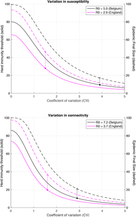
 In more complex cases (such as the variable connectivity with dynamic CV or assortative mixing) HIT curves can be approximated numerically. Figure 3 shows the expected downward trends in HIT and the sizes of the respective unmitigated epidemics for SARS-CoV-2 without reinfection (σ = 0) as the coefficients of variation are increased (here we adopt gamma distributions; for robustness of the trends to other distributions see Gomes et al9). Values of R0 and CV estimated for our study countries are overlaid to mark the respective HIT and final epidemic sizes. While herd immunity is expected to require 60-80% of a homogeneous population to have been infected, at the cost of infecting almost the entire population if left unmitigated, given an R0 between 2.5 and 5, these percentages drop to the range 10-20% when CV is roughly between 1.5 and 4.
Curves generated with the SEIR model (Equation 1-4) assuming values of R0 estimated for the study countries (Extended Data Tables 1 and 2) assuming gamma-distributed: susceptibility (top); connectivity (bottom) with constant CV. Herd immunity thresholds (solid curves) are calculated according to the formula 1 − (1/R0)1/(1+CV2) for heterogeneous susceptibility and 1 − (1/R0)1/(1+2CV2) for heterogeneous connectivity. Final sizes of the corresponding unmitigated epidemics are also shown (dashed).
When acquired immunity is not 100% effective (σ > 0) HITs are relatively higher (Extended Data Figure 3). However, there is an upper bound for how much it is reasonable to increase σ before the system enters a qualitatively different regime. Above σ = 1/R0 – the reinfection threshold10,11– infection becomes stably endemic and the HIT concept no longer applies. Respiratory viruses are typically associated with epidemic dynamics below the reinfection threshold, characterized by seasonal epidemics intertwined with periods of low detection.
Curves in the main panels generated with the SEIR model (Equation 1-4) assuming R0 = 3 and gamma-distributed susceptibility (top) or connectivity (bottom) with constant CV. Efficacy of acquired immunity is captured by a reinfection parameter σ, potentially ranging between σ = 0 (100% efficacy) and σ = 1 (0 efficacy). This illustration depicts final sizes of unmitigated epidemics and associated HIT curves for 6 values of σ: σ = 0 (black); σ = 0.1 (green); σ = 0.2 (blue); σ = 0.3 (magenta); σ = 1/3 (red); and σ = 0.4 (orange);. Above σ = 1/R0(reinfection threshold (Gomes et al 2004; 2016)) the infection becomes stably endemic and there is no herd immunity threshold. Representative epidemics of the regime σ ≤ 1/R0 are shown on the right while the regime σ > 1/R0 is illustrated on top. All depicted dynamics are based on the rightmost CVs represented on the main panel.
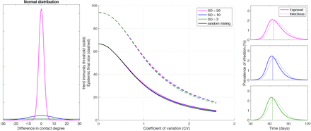
Individual variation in exposure, in contrast with susceptibility, accrues from complex patterns of human behaviour which have been simplified in our basic model. To explore the scope of our results we generalised the models by relaxing some key assumptions. First, we allowed connectivity distributions to change in shape (not only scale) when subject to social distancing (Figure 1, bottom panels). Second, we enable mixing to be assortative in the sense that individuals contact predominantly with those of similar connectivity (Methods). Formally, an individual with connectivity x, rather than being exposed uniformly to individuals of all connectivities y, has contact preferences described by a normal distribution on the difference y − x. We find this modification to have negligible effect on HIT (Extended Data Figure 4).
Curves in central panel generated with the SEIR model (Equation 1-4) assuming R0 = 3 and gamma-distributed connectivity. Assortative mixing is implemented by imposing a normal distribution for contact preferences such that individuals contact preferentially with those with the similar contact degree (left). This illustration used normal distributions with standard deviation SD = 50 (green); SD = 10 (blue); and SD = 2 (magenta). More assortative mixing leads to more skewed epidemics. Herd immunity thresholds were calculated numerically as the percentage of the population no longer susceptible when new outbreaks are effectively prevented (approximately when the exposed fraction crosses the peak in the absence of mitigation). Final sizes of the corresponding unmitigated epidemics are also shown. Representative epidemics are depicted on the right based on the rightmost CVs represented on the main panel (with vertical lines marking the point when herd immunity is achieved).
Herd immunity thresholds and seroprevalence at sub-national levels
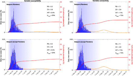
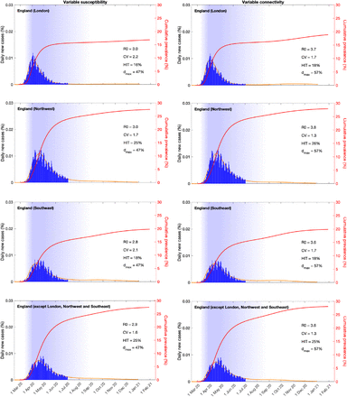
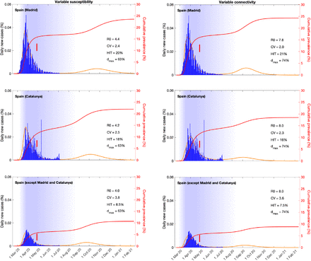
As countries conduct immunological surveys to assess the extent of exposure to SARS-CoV-2 in populations it is of practical importance to understand how HIT may vary across regions. We have redesigned our analyses to address this question. Series of daily new cases in 4 European countries (Belgium, England, Portugal and Spain) were stratified by region. Fitting the models simultaneously to the multiple series enabled the estimation of local parameters (R0 and CV) while the effects of NPIs were estimated at country level. Extended Data Figures 5-8 show how the modelled epidemics fit the regional data and include an additional metric to describe the cumulative infected percentage. These model projections are comparable to data from seroprevalence studies such as in Spain12. In addition to their practical utility these results begin to unpack some of the variation in HIT within countries: Belgium (9.4-11%), England (16-26%), Portugal (7.1-9.9%) and Spain (7.5-21%). The sub-national stratification has also enabled the application of the models to countries where the epidemic was sufficiently asynchronous across regions to compromise the ability of the models to fit the aggregate data (Portugal and Spain).
Suppressed wave and subsequent dynamics in Flanders and the rest of Belgium, with individual variation in susceptibility (left) or exposure (right). Blue bars are daily new cases. Shades represent social distancing (intensity reflected in shade density). Susceptibility or exposure factors implemented as gamma distributions. Consensus parameter values (Methods): δ = 1/4 per day; γ = 1/4 per day; and ρ = 0.5. Fraction of infected individuals identified as positive (reporting fraction): 0.06. Basic reproduction number, coefficients of variation and social distancing parameters estimated by Bayesian inference as described in Methods (estimates in Extended Data Table 1 and 2). Curves represent mean model predictions from 104 posterior samples. Orange shades represent 95% credible intervals. Red curves represent cumulative infected percentages.
Suppressed wave and subsequent dynamics in London, Northwest, Southeast and the rest of England, with individual variation in susceptibility (left) or exposure (right). Blue bars are daily new cases. Shades represent social distancing (intensity reflected in shade density). Susceptibility or exposure factors implemented as gamma distributions. Consensus parameter values (Methods): δ = 1/4 per day; γ = 1/4 per day; and ρ = 0.5. Fraction of infected individuals identified as positive (reporting fraction): 0.024. Basic reproduction number, coefficients of variation and social distancing parameters estimated by Bayesian inference as described in Methods (estimates in Extended Data Table 1 and 2). Curves represent mean model predictions from 104 posterior samples. Orange shades represent 95% credible intervals. Red curves represent cumulative infected percentages.
Suppressed wave and subsequent dynamics in the North and Centre regions versus the rest of Portugal, with individual variation in susceptibility (left) or exposure (right). Blue bars are daily new cases. Shades represent social distancing (intensity reflected in shade density). Susceptibility or exposure factors implemented as gamma distributions. Consensus parameter values (Methods): δ = 1/4 per day; γ = 1/4 per day; and ρ = 0.5. Fraction of infected individuals identified as positive (reporting fraction): 0.09. Basic reproduction number, coefficients of variation and social distancing parameters estimated by Bayesian inference as described in Methods (estimates in Extended Data Table 1 and 2). Curves represent mean model predictions from 104 posterior samples. Orange shades represent 95% credible intervals. Red curves represent cumulative infected percentages.
Suppressed wave and subsequent dynamics in Madrid, Catalunya and the rest of Spain, with individual variation in susceptibility (left) or exposure (right). Blue bars are daily new cases. Shades represent social distancing (intensity reflected in shade density). Susceptibility or exposure factors implemented as gamma distributions. Consensus parameter values (Methods): δ = 1/4 per day; γ = 1/4 per day; and ρ = 0.5. Fraction of infected individuals identified as positive (reporting fraction): 0.06. Basic reproduction number, coefficients of variation and social distancing parameters estimated by Bayesian inference as described in Methods (estimates in Extended Data Table 1 and 2). Curves represent mean model predictions from 104 posterior samples. Orange shades represent 95% credible intervals. Red curves represent cumulative infected percentages and vertical red segments mark seroprevalences (95% CI) according to a recent study12.
Discussion
The concept of herd immunity was developed in the context of vaccination programs13,14. Defining the percentage of the population that must be immune to cause infection incidences to decline, HITs constitute useful targets for vaccination coverage. In idealized scenarios of vaccines delivered at random and individuals mixing at random, HITs are given by a simple formula (1 − 1/R0) which, in the case of SARS-CoV-2, suggests that 60-80% of randomly chosen subjects of the population would need be immunized to halt spread considering estimates of R0 between 2.5 and 5. This formula does not apply to infection-induced immunity because natural infection does not occur at random. Individuals who are more susceptible or more exposed are more prone to be infected and become immune, providing greater community protection than random vaccination15. In our model, the HIT declines sharply when coefficients of variation increase from 0 to 2 and remains below roughly 20% for more variable populations. The magnitude of the decline depends on what property is heterogeneous and how it is distributed among individuals, but the downward trend is robust as long as susceptibility or exposure to infection are variable (Figure 3 and Extended Data Figures 4) and acquired immunity is efficacious enough to keep transmission below the reinfection threshold (Extended Data Figure 3).
Several candidate vaccines against SARS-CoV-2 are showing promising safety and immunogenicity in early-phase clinical trials16,17, although it is not yet known how this will translate into effective protection. We note that the reinfection threshold10,11 informs not only the requirements on naturally acquired immunity but, similarly, it sets a target for how efficacious a vaccine needs to be in order to effectively interrupt transmission. Specifically, given an estimated value of R0 we should aim for a vaccine efficacy of 1 − 1/R0 (60% or 80% if R0 is 2.5 or 5, respectively), which seems to be materialising according to preliminary results from phase 3 trials.
Heterogeneity in the transmission of respiratory infections has traditionally focused on variation in exposure summarized into age-structured contact matrices. Besides overlooking differences in susceptibility given exposure, the aggregation of individuals into age groups reduces coefficients of variation. We calculated CV for the landmark POLYMOD matrices18,19 and obtained values between 0.3 and 0.5. Recent studies of COVID-19 integrated contact matrices with age-specific susceptibility to infection (structured in three levels)20 or with social activity (three levels also)21 which, again, resulted in coefficients of variation less than unity. We show that models with coefficients of variation of this magnitude would appear to differ only moderately from homogeneous approximations when compared with our estimates, which are consistently above 1 in England and above 2 in Belgium, Portugal and Spain. In contrast with reductionist procedures that aim to reconstruct variation from correlate markers left on individuals (such as antibody or reactive T cells for susceptibility, or contact frequencies for exposure), we have embarked on a holistic approach designed to infer the whole extent of individual variation from the imprint it leaves on epidemic trajectories. Our estimates are therefore expected to be higher and should ultimately be confronted with more direct measurements as these become available. Adam at et22 conducted a contact tracing study in Hong Kong and estimated a coefficient of variation of 2.5 for the number of secondary infections caused by individuals, attributing 80% of transmission to 20% of cases. This statistical dispersion has been interpreted as reflecting a common pattern of contact heterogeneity which has been corroborated by studies that specifically measure mobility23. According to our inferences, 20% of individuals may be responsible for 47-94% infections depending on model and country. In parallel, there is accumulating evidence of individual variation in the immune system’s ability to control SARS-CoV-2 infection following exposure24,25. While our inferences serve their purpose of improving accuracy in model predictions, diverse studies such as these are necessary for developing interventions targeting individuals who may be at higher risk of being infected and propagating infection in the community.
Country-level estimates of R0 reported here (Figures 1, 2) are in the range 3-5 when individual variation in susceptibility is factored and 4-9 when accounting for variation in connectivity. The homogeneous version of our models would have estimated R0 around 2.7 and 3.7, in line with other studies26. Estimates for England suggest lower baseline R0 and lower CV in comparison with Belgium. The net effect is a slightly higher HIT in England which nevertheless we estimate around 25-27% depending on characteristics of the individual variation. NPIs reveal less impact when heterogeneity is contemplated (37-60%), appearing to inflate and agree with Flaxman et al26 when homogeneity assumptions are made (66-78%), although this does not affect the HIT which relates to pre-pandemic societies.
More informative than reading these numbers, however, is to look at simulated projections of how cases may unfold over future months (Figures 1, 2). In both countries, when individual variation is considered, we foresee HIT being achieved and the COVID-19 epidemic being mostly resolved by the end of 2020. Under the homogeneous approximation, however, epidemic potential appears to justify considerations of second lockdowns to flatten epidemic curves. Determining the level of confidence on either scenario is highly relevant to policy decisions and hence of central importance to public health. According to the Akaike information criterion (Extended Data Table 5) data favours the models that account for individual variation and a more natural resolution for the pandemic. Models that account for individual variation in susceptibility score particularly well and amongst those that account for variation in exposure those that allow this variation to reduce with social distancing perform better.
Displays the maximum Loglikelihood obtained for each combination of model and data partitioning for each country, as well as the Akaike information criterion. Models are labelled by a sort name as follows: homog (homogenous); hetsus (heterogeneity in susceptibility); hetcon (heterogeneity in connectivity with constant CV); hetdyn (heterogeneity in connectivity with dynamic CV).
Looking back, we conclude that NPIs had a crucial role in halting the growth of the initial wave between February and April irrespective of individual variation. Although the most extreme lockdown strategies may not be sustainable for longer than a month or two, they proved effective at preventing overshoot, keeping cases within health system capacities, and may have done so without impairing the development of herd immunity.
METHODS
Model structure and underlying assumptions
The model presented here is a differential equation SEIR model, where susceptible individuals become exposed at a rate that depends on their susceptibility, the number of potentially infectious contacts they engage in, and the total number of infectious people in the population per time unit. Upon exposure, individuals enter an asymptomatic incubation phase, during which they slowly become infectious27-30. Thus, infectivity of exposed individuals is made to be 1/2 of that of infectious ones (ρ = 0.5). After a few days, individuals develop symptoms – on average 4 days after the exposure to the virus (δ = 1/4) – and thus become fully infectious31-33. They recover, i.e., they are no longer infectious 4 days after that (γ = 1/4), on average34.
Efficacy of acquired immunity
We conducted the core of our analysis under the assumption that no reinfection occurs after recovery due to acquired immunity (σ = 0). To analyse the sensitivity of these results to leakage in immune response (σ > 0) we calculated herd immunity thresholds (HIT) as a function of coefficients of variation (CV) for different values of σ. The results displayed in Extended Data Figure 3 confirm the expectation that as the efficacy of acquired immunity decreases (σ increases) larger percentages of the population are infected before herd immunity is reached. Less intuitive is that there is an upper bound for how much it is reasonable to increase σ before the system enters a qualitatively different regime – the reinfection threshold10,11 (σ = 1/R0) – above which infection becomes stably endemic and the notion of herd immunity threshold no longer applies. Respiratory viruses are typically associated with epidemics dynamics below the reinfection threshold.
Effective reproduction number
The effective reproduction number (Reff also denoted by Re or Rt by other authors) is a time-dependent quantity which we calculate as the incidence of new infections divided by the total number of active infections (affected by ρ for individuals in E) multiplied by the average duration of infection (also affected by ρ for individuals in E)

Assortative mixing
In the main text we assumed random mixing among individuals, but human connectivity patterns are assortative due societal structures and human behaviours. To explore the sensitivity of our results to deviations from random mixing, we develop an extended formalism that allows individuals to connect preferentially with those with similar connectivity, formally λ(x) = (β/N)(∫ y h(y − x)[ρE(y) + I(y)] dy/∫ yg(y) dy), where h(y − x) is a normal distribution on the difference between connectivity factors (Extended Data Figure 2).
Non-pharmaceutical interventions
We implemented non-pharmaceutical interventions (NPI) as a gradual decrease in viral transmissibility in the population and thus a lowering of the controlled and effective reproduction numbers (Rc and Reff). Once containment measures are put in place in each country, we postulate it takes 21 days until the maximum effectiveness of social distancing measures is reached, approximately linearly. In the simulations presented throughout we have held this condition (maximum “lockdown” efficacy) for Tmax days, where Tmax is estimated for each study country in countrywide analyses and fixed at 30 in regional analyses. Eventually, lockdowns were lifted and social distancing measures progressively relaxed. This relaxation is implemented linearly over a period of Tlift days, which is also estimated. We note however that the estimation of epidemiological parameters is not affected by the shape assumed for the relaxation of interventions beyond the date of the last data point (June 11th in Belgium and July 1st in England). In particular, assuming that social distancing measures remained constant from these dates onwards, for example, would make no difference to the estimated parameters.
Bayesian Inference
The model laid out above is amenable to theoretical exploration as presented in the main manuscript and provides a perfect framework for inference. Fundamentally, to be able to reproduce the inception of any epidemic, we would need to estimate when local transmission started to occur (t0), and the pace at which individuals infected each other in the very early stages of the epidemic (R0). All countries, to different extents and at different timepoints of the epidemic, enforced some combination of social distancing measures. To fully understand the interplay between herd immunity and the impact of NPIs, we then set out to estimate the time at which social distancing measures started to have an impact on daily incidence  , what their maximum efficacy (dmax) was and how long it lasted (Tmax), a parameter used to determine the rate at which contacts resume as restrictions are lifted (Tlift, which more specifically represents the time it would take to reach pre-pandemic contact intensity should the lifting of restricting have linear effect), the basic reproduction number (R0) and what the underlying variance in heterogeneity is for susceptibility or exposure to infection.
In order to preserve identifiability, we made two simplifying assumptions: (i) the fraction of infectious individuals reported as COVID-19 cases (reporting fraction) is constant throughout the study period and is comparable between countries proportionally to the number of tests performed per person; (ii) local transmission starts (t0) when countries/regions report 1 case per 5 million population in one day. To calculate the reporting rates, we used the Spanish national serological survey12 as a reference and divided the total number of reported cases up to May 11th by the estimated number of people that had been exposed to the virus. This gives us a reporting rate for Spain around 6%. Unfortunately, there are no other national serological surveys that could inform the proportion of the population infected in other countries, so we had to extrapolate the reporting rate for those. Assuming the reporting rate is highly dependent on the testing effort employed in each country, reflected in the number of tests per individual, we estimate the reporting rate by scaling the reporting rate recorded in Spain according to the ratio of PCR tests per person in other countries relative to the Spanish reference of 0.9 tests per thousand people (https://ourworldindata.org/coronavirus-testing). This produced estimated case reporting rates (ratio of reported cases to infections) of 9% for Portugal, 6% for Belgium (and Spain) and 2.4% for England.
Whist national case and mortality data is easily available for most countries, more spatially resolute data is difficult to find in the public domain. Thus, we restricted our analysis to countries for which disaggregated regional case data was easily available. We collected the data at two time points. First, we compiled all available data from the day the countries started reporting COVID-19 cases to the initial collection date (May 20th) and later collated available data from May 21st to July 10th.
Parameter estimation was performed with the software MATLAB, using PESTO (Parameter EStimation Toolbox)35, and assuming the reported case data can be accurately described by a Poisson process. We first fixed the beginning of local transmission (parameter t0) in each data series as the day in which reported cases surpassed 1 in 5 million individuals. Next, we optimized the model for the set of parameters  by maximizing the logarithm of the likelihood (LL) (Equation 10) of observing the daily reported number of cases in each country
 in which y(k, θ) is the simulated model output number of COVID-19 cases at day k (with respect to t0), and n is the total number of days included in the analysis for each country.
To ensure that the estimated maximum is a global maximum, we performed 50 multi-starts optimizations, and selected the combination of parameters resulting in the maximal Loglikelihood as a starting point for 104 Markov Chain Monte-Carlo iterations. From the resulting posterior distributions, we extract the median estimates for each parameter and the respective 95% credible intervals for the set of parameters. We used uniformly distributed priors with ranges {1-9, 0.0025-8,1-60, 0-0.7,1-90,60-1000}.
When fitting the model to disaggregated data, we follow the procedure outlined above but fix Tmax = 30 days, Tllift = 120 days and estimate region-specific R0 and CV, with common  and dmax.
The countrywide fitting procedure was applied to 2 countries (Belgium and England) and repeated for each of the 4 model variants considered here (homogeneous, heterogeneous susceptibility, heterogeneous connectivity with constant CV, and heterogeneous connectivity with CV reducing in proportion to social distancing). Our study included two more countries (Portugal and Spain), where countrywide analyses could not be performed due to the epidemic being geographically desynchronised. We implemented stratified analyses on all 4 countries. In the fitting procedures using sub-national data, we assumed regions had the same start date for interventions that mitigate transmission  , and that these measures produced the same maximum impact on transmission (dmax) everywhere. Thus, the only region-specific parameters to be estimated are
 . Parameter estimates obtained from each of the model variants are displayed in Extended Data Table 1 (heterogeneity in susceptibility), Extended Data Table 2 (heterogeneity in connectivity with constant CV), Extended Data Table 3 (heterogeneity in connectivity with dynamic CV) and Extended Data Table 4 (homogeneous model), are comparable to those obtained in other studies7,26,37-40. Finally, we apply the Akaike information criterion (AIC) for each estimation procedure to inform on the quality of each model’s fit to the datasets of reported cases (Extended Data Table 5). In all cases, heterogeneous models are preferred over the homogeneous approximation. The three heterogeneous models are roughly equally well supported by the data used in this study. Further research should complement this with discriminatory data types and hybrid models to enable the integration of different forms of individual variation.
Data and code availability
Datasets are publicly available at the respective national ministry of health websites (41-45). Core models implemented in MATLAB available from: https://github.com/mgmgomes1/covid
Author contributions
M.G.M.G. conceived the study. R.A. and R.M.C. and M.G.M.G. performed the analyses. All authors interpreted the data and wrote the paper.
Competing interests
The authors declare no competing interests.
Acknowledgements
We thank Jan Hasenauer and Antonio Montalbán for helpful discussions concerning statistical inference and mathematics, respectively. R.M.C. and M.U.F. receive scholarships from the Conselho Nacional de Desenvolvimento Científico e Tecnológio (CNPq), Brazil.
Footnotes
More flexible implementation of NPI in countrywide analyses.


