
Abstract
Importance: Monitoring health systems during and after natural disasters, epidemics, or outbreaks is critical for guiding policy decisions and interventions. When the effects of an event are long-lasting and difficult to detect in the short term, the accumulated effects can be devastating.
Objective: We aim to leverage the improved access to mortality data to develop data-driven approaches that can help monitor health systems and quantify the effects on mortality of natural disasters, epidemics, or outbreaks.
Design, Setting, and Participants: To demonstrate the utility of our approach we conducted several retrospective time-series analyses of mortality assessment after natural disasters. We obtained individual-level mortality records from the Department of Health of Puerto Rico from January 1985 to May 2020 to study the effects of hurricanes Hugo, Georges, and María in September 1989, September 1998, and September 2017, respectively. Further, we obtained daily mortality counts from Florida, New Jersey, and Louisiana’s Vital Statistic systems from January 2015 to December 2018, January 2007 to December 2015, and January 2003 to December 2006, respectively, to study the effects of hurricanes Irma in 2017, Sandy in 2013, and Katrina in 2005. Finally, we obtained individual-level mortality data from the Cook county, IL, medical examiners office, and state-specific weekly mortality counts from the Center for Disease Control and Prevention to assess the effect of the COVID-19 pandemic on the US health system.
Exposures: Hurricanes María, Georges, and Hugo in Puerto Rico, Irma in Florida, Sandy in New Jersey, and Katrina in Louisiana, the Chikungunya outbreak in Puerto Rico, and the COVID-19 pandemic in the United States.
Main Outcomes: We estimate and provide uncertainty assessments for percent increase from expected mortality, estimated excess deaths, and difference across groups.
Results: We found that the death rate increase in Puerto Rico after María and Georges was substantially higher than the other hurricanes we examined. Further, we find that excess mortality in the US was already above 100,000 on May 9, 2020, with over 58% of these occurred in New York, New Jersey, Massachusetts, and Pennsylvania, and that effects of this pandemic were worse for elderly black individuals compared to whites of the same age.
Conclusions and Relevance: Our approach can be used to monitor or assess health systems by estimating increased mortality rates and excess deaths from mortality records.
Key Points
Question: Can we estimate excess mortality and provide accurate uncertainty assessments from vital statistics data?
Findings: We developed statistical methodology that accounts for key sources of variability and provides accurate estimates and their standard errors for excess mortality. We applied the approach to datasets from several US states including periods affected by hurricanes and epidemics. We found an elevated and persistent increase in mortality after hurricanes in Puerto Rico that was substantially higher than in other US states. We also found that excess mortality in the US during the COVID-19 pandemic reached 100,000 by May 9, 2020. Finally, we found significant differences in the effects of this pandemic across racial groups in the US.
Meaning: Data-driven approaches can help monitor health systems and quantify the effects on mortality of natural disasters, epidemics, or outbreaks.
1 Introduction
Hurricane María made landfall in Puerto Rico on September 20, 2017, interrupting the water supply, electricity, telecommunications networks, and access to medical care[1, 2]. Two weeks after the hurricane, the official death count stood at 16[3]. However, groups that ostensibly had access to death counts for September and October from the demographic registry of Puerto Rico estimated additional deaths to be in excess of 1,000[4, 5, 6, 7], raising concerns that Puerto Rico was in the midst of a public health crisis. After several lawsuits and pressure from domestic and international media due to a survey-based study that reported a higher death count [8], the official death toll was revised to 2,975 in August 2018, based on a study commissioned by the government.
More recently, the limited capacity to perform molecular tests has raised concerns that COVID-19 cases are under-reported in several jurisdictions in the United States and across the world. Simultaneously, polls show that a substantial proportion of the US population believes that reported COVID-19 fatalities are inflated [9]. Estimating excess mortality provides a way to measure the impact of the epidemic, even in the presence of inaccurate reporting.
The main goal of our method is to determine if an observed death count for a given demographic and period is unusually high. This can alert government officials and policymakers that an intervention is required. The uncertainty associated with count data, such as daily deaths, are typically accounted for with Poisson models[10, 11]. However, these models do not account for year-to-year variability that may be due to natural, possibly correlated, stochastic variation. Ignoring this source of correlated variation can lead to underestimates of the uncertainty associated with mortality excess estimates.
To demonstrate the utility of our approach, we provide a detailed picture of the effect Hurricane María had on mortality in Puerto Rico and compare these to those observed in Hugo and Georges, two previous hurricanes in Puerto Rico, Katrina in Louisiana, Irma in Florida, and Sandy in New Jersey. We also used our approach to search for unusually high mortality rates during the last 35 years in Puerto Rico. We then apply our method to recently released state-level data by the Center for Disease Control and Prevention (CDC) and compare the excess deaths during the COVID-19 epidemic to those from the 2018 flu season. We also compare the excess mortality between racial groups in Cook County, Illinois, the only county we are aware of that is currently releasing up to date medical examiner records. Finally, we propose a data-driven index that does not require complete data nor an estimate of population size, which is useful in cases in which estimating population size is challenging, thus making real-time estimates less reliable. We make our method available through the excessmort R package.
2 Methods
2.1 Mortality Data
For Puerto Rico, we requested individual-level mortality information with no personal identifiers from the Department of Health of Puerto Rico and obtained individual records including date, gender, age, and cause of death from January 1985 to May 2020. We also obtained daily death counts from Florida, New Jersey, and Louisiana’s Vital Statistic systems from January 2015 to December 2018, January 2007 to December 2015, and January 2003 to December 2006, respectively. Further, we obtained mortality data made public on May 29, 2020, by the CDC[12]. This dataset included weekly estimates of death counts for each state for the period of January 2017 and May 2020. Finally, we obtained individual-level mortality data from Cook County, IL, medical examiner office[13], which included demographic information for each death including age, sex, and race.
2.2 Population Estimates
Yearly population estimates for Puerto Rico were obtained from the Puerto Rico Statistical Institute. Yearly population estimates for other US states were obtained from the US Census bureau. To obtain an estimate of the population displacement after Hurricane María in Puerto Rico, we use population proportion estimates from Teralytics – a company that works with governments and private clients to assess human movement by partnering with mobile network operators. This company provided daily population proportion estimates relative to an undisclosed baseline from May 31, 2017, to April 30, 2018. This was based on all subscribers of a major, undisclosed, telecommunications company in Puerto Rico. Due to structural damage post-Hurricane Maria, proportion estimates for the four weeks after the storm were not provided. We imputed missing data with linear interpolation of observed values. We then computed population estimates by multiplying the US census population estimate on July 19, 2017, Teralytics baseline date, times the aforementioned proportions, and obtained smooth values using local regression (Supplementary Figure 1).

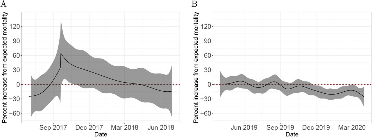
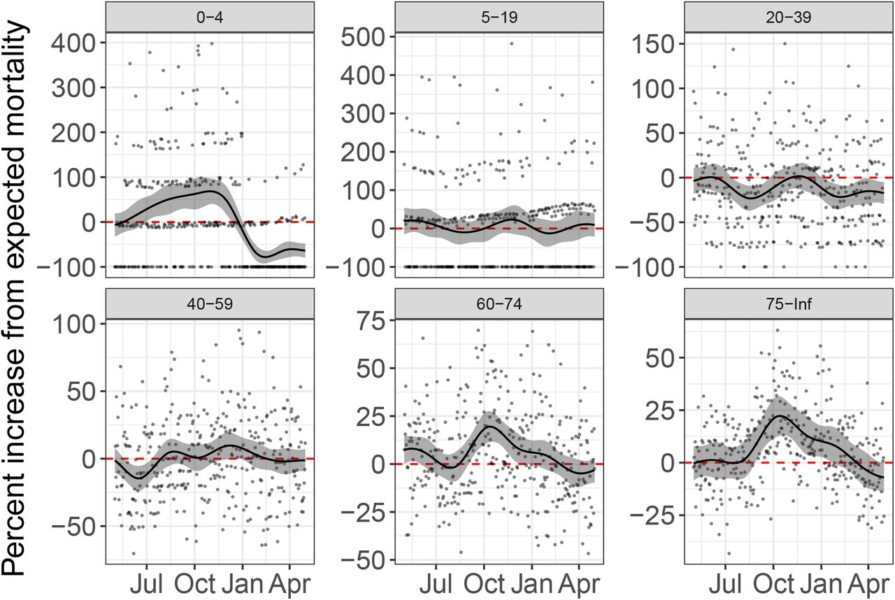
Estimated event effects as percent increase over expected mortality. A) Comparison of six hurricanes. B) Estimated increase and point-wise confidence intervals during the Chikungunya epidemic in Puerto Rico. C) Estimated increase and confidence interval for the the United States from January 2017 through May 2020.
2.3 Statistical model
Extending the work developed for monitoring outbreaks [14, 15, 16, 17] we modeled death counts with the following mixed model
 with μt the expected number of deaths at time t for a typical period, 100 × f(t) the percent increase at time t due to an unusual event, εt a time series of auto-correlated random variables representing natural variability, and T the total number of observations. The expected counts μt can be further decomposed into
 with Nt the population at time t, α(t) a slow moving trend that accounts for changes such as the improved health outcomes we have observed during the last 20 years (Supplementary Figure 2A), s(t) a yearly periodic function representing a seasonal trend (Supplementary Figure 2B), and w(t) is a day of the week effect. We refer to f as the event effect and assume f (t) = 0 for typical periods not affected by a natural disaster or outbreak. Our model permits non-continuities in f (t) to account for sudden direct effects caused by natural disasters. Note that we can conveniently represent excess deaths at time t as μt × f (t) and compute excess deaths for a time period by just adding these up for the t’s in the interval of interest. We assume the vector [ε1, …, ε T]T follows a multivariate normal distribution with mean 1 and variance-covariance matrix Σ determined by an auto-regressive (AR) process of order p. In practice, obtaining Maximum Likelihood Estimates (MLE) for this model is not straight-forward, in particular because the flexibility in f (t) and Σ makes the model non-identifiable in practice. To overcome this challenge, we implemented a three step approach that works well in practice, as demonstrated both by simulation and empirical validation. Further details and validation of our model and estimation procedure is provided in the Supplementary Material. The code to reproduce our analysis as well as the R package implementing the methods are available at https://github.com/rafalab/excess-mortality-paper and https://github.com/rafalab/excessmort, respectively.

Cumulative excess mortality estimates. A) Daily excess death estimates and 95% confidence intervals for events in Puerto Rico starting on September 20, 2017, September 21, 1998, July 14, 2014, and March 1, 2020 for Hurricane María, Hurricane Georges, the Chikungunya epidemic, and the COVID-19 pandemic, respectively. B) Estimated cumulative excess mortality and reported COVID-19 cumulative deaths in the United States. C) State-specific cumulative excess death estimates from March 1, 2020 to May 16, 2020, the period associated with the COVID-19 pandemic, plotted against the excess mortality estimates from December 10, 2017 to February 24, 2018, the period associated with the 2018 flu season. The identity line is represented in red and separates states in which the increase in mortality was higher during COVID-19 from those in which the increase in mortality was higher during the 2018 flu season.
3 Results
3.1 Detecting and quantifying indirect effects after hurricanes
Using our approach, we found that the death rate in Puerto Rico increased by 73% (95% CI: 58% to 87%) the days after hurricane María made landfall. The increased death rate persisted until March 2018 (Figure 1A, Supplementary Figure 3). To understand if such a large and sustained increase is common after the passage of a hurricane, we examined mortality counts in Louisiana after Katrina, New Jersey after Sandy, Florida after Irma as well as two other hurricanes in Puerto Rico, Hugo in 1989 and Georges in 1998. Although not as severe, a similar pattern to María was observed for Georges in 1998 when the death rate increased by 36% (95% CI: 24% to 48%) the days after landfall and an increased death rate persisted until December 1998 (Figure 1A, Supplementary Figure 3). The effects of Katrina on Louisiana were much more direct. On August 29, 2005, the day the levees broke, there were 834 deaths, which translates to an increase in death rate of 689% (not shown in Figure 1A). However, the increase in mortality rates for the months following this catastrophe was substantially lower than in Puerto Rico after María and Georges. None of the other hurricanes examined had direct or indirect effects nearly as high as in Puerto Rico (Figure 1A, Supplementary Figure 3).

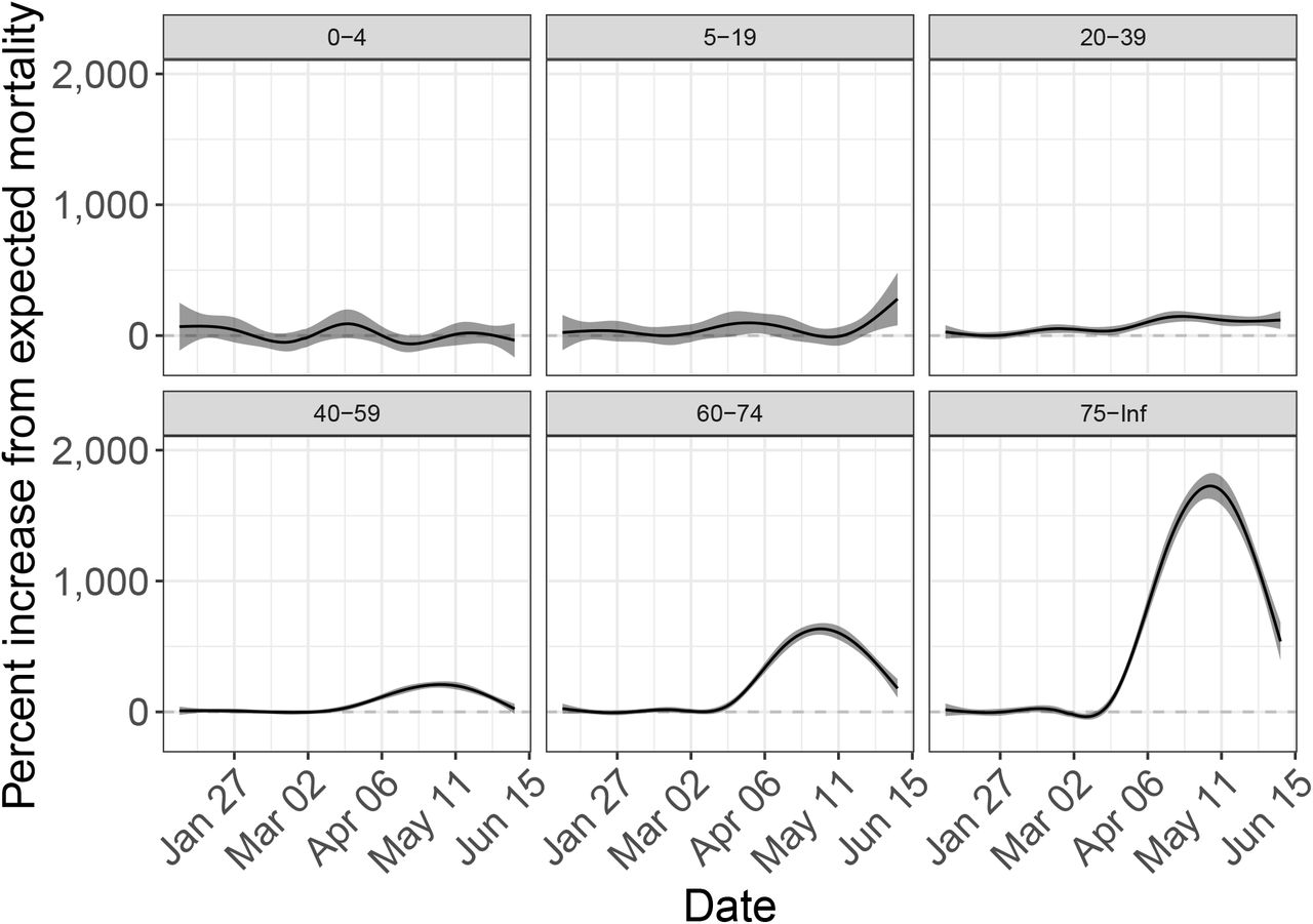
Comparison of estimated percent increase in mortality in Cook county, Illinois, for individuals above 40 between whites and blacks with corresponding 95% confidence intervals. A) 40 to 59 age group. B) 60 to 74 age group. C) 75 and over age group.
3.2 Quantifying the effects of epidemics
Our approach can also be used to detect and quantify the effects of epidemics or outbreaks. As an example, we fit our model to Puerto Rico mortality data from 1985 to 2020 and, apart from the hurricane seasons mentioned in the previous section, we detected an unusual increase in mortality rates from July 2014 to February 2015. This period coincides with the 2014-2015 Chikungunya outbreak [18, 19] (Figure 1B). The effects were particularly strong for individuals over 60 years and for the 0 to 4 years age group. (Supplementary Figure 4).

Cause-specific mortality index. The solid-black line corresponds to the percent change in proportion of mortality,  , attributable to a cause of interest. The shaded area represents a 95% confidence interval for
  . A) Bacterial infections mortality index defined as ICD10 codes between A00 and A79 for the dates around Hurricane María. B) Respiratory diseases mortality index defined as ICD10 codes between J00 and J99 for the dates around the COVID-19 pandemic in Puerto Rico.
Although mortality records for the period of the COVID-19 pandemic are not yet complete, the CDC has implemented a correction to the most recent counts and is making weekly state-level data from January 2017, to May 2020, publicly available [12]. We fit our model to these data for each state and our event effect estimates detect the pandemic for several states, as well as the 2018 flu epidemics (Supplementary Figure 6). By aggregating the results for the entire United States we confirm that the COVID-19 pandemic had a substantially larger impact than the 2018 flu season (Figure 1C).
3.3 Excess mortality estimates
Once we have fit our model, we can compute excess mortality estimates for any period as well as standard errors that take into account sampling and natural variation. We used the estimated parameters from the Puerto Rico data to compute excess deaths for the 365 days following hurricanes Georges, and Maria. We also computed these quantities for the 365 days following the start of the detected effects from the 2014 Chikungunya outbreak. Finally, we computed excess deaths in Puerto Rico during the COVID-19 pandemic, specifically from March 1, 2020, to April 15, 2020, the last day for which the death registry has complete data (typically, it takes 90 days for 99% of deaths to be registered).
For María the excess death curve grew for over six months after landfall, with a point estimate on March 20, 2018, six months after landfall, of 3,200 (95% CI: 2,800 to 3,600), and for Georges, the excess death curve grew for over three months after landfall, with a point estimate on December 21, 1998, three months after landfall, of 1,200 (95% CI: 950 to 1,500) (Figure 2A). The period of July 14, 2014, to February 20, 2015, associated with a Chikungunya outbreak was also identified to have unusually high mortality rates. However, we also noted a decrease in cumulative deaths for several months after February 20, 2015, consistent with a harvesting effect [20, 21]. A year after the start of the Chikungunya epidemic, on July 14, 2015, we observe a point estimate for excess mortality of 975 (95% CI:400 to 1,550) (Figure 2A). We note that from March 1, 2020, to April 15, 2020, associated with the COVID-19 pandemic, no effect is detected.
Next, using the CDC data we computed excess mortality for the period of the COVID-19pandemic for which we have data, specifically for the week ending on March 15, 2020, to the week ending on May 16, 2020. When we compared these numbers to the reported numbers of COVID-19 deaths [22], we found a difference of 32,257 (95% CI: 30,211 to 34,303) deaths (Figure 2B, Table 1). Further, we found that excess deaths in the US were already above 100,000 on May 9, 2020. We also note that in the US, the number of excess deaths during the COVID-19 pandemic is much larger than the 2018 flu season, although this is not true for all states (Figure 2C, Table 1, Supplementary Figure 5). We also note that 58% of the cases come from the four northeast states: New York, New Jersey, Massachusetts, and Pennsylvania (Supplementary Figure 6). We note that Connecticut was not included in the analysis due to missing data.
Excess mortality estimates from March 1, 2020 to May 16, 2020 (COVID-19) and December 10, 2017 to February 24, 2018 (2018 Flu). The standard deviation for excess mortality for these periods is included in parenthesis. The states are ordered by the per-million excess mortality rate. Connecticut and North Carolina are excluded due to missing data. Numbers for New York do not include New York City which is listed separately.
3.4 Across group comparisons
At the time of writing, the Cook County Medical Examiner’s Office was making up-to-date records available online including demographic information for each individual. This office investigates any human death in Cook County that falls within the category of diseases constituting a threat to public health, among other circumstances[13]. If we consider to be the expected number of deaths recorded by the Medical Examiner’s Office, we can fit our model and interpret f (t) as the percent increase in deaths examined by this office. We fit the model to these data and observed the effects of the COVID-19 pandemic, in particular among individuals over 75. However, a persistent increase in mortality above normal levels is observed for individuals above 40 (Supplementary Figure 7). Furthermore, we found a difference in the effect between white and black individuals in March and April (Figure 3). Among those between 40 and 59 years of age, the percent increase in medical examiner death rates for Cook county was as high as 188% (95% CI: 150% to 226%) and 101% (95% CI: 68% to 134%) on April 23 for blacks and whites, respectively. Furthermore, for the 60 to 74 age group we observed a percent increase of 628% (95% CI: 560% to 696%) and 398% (95% CI: 345% to 451%) on the same date, respectively. Finally, the percent increase for individuals 75 years and older on the same date was 2,193% (95% CI: 1,996% to 2,389%) and 1,062% (95% CI: 974% to 1,150%), respectively, another statistically significant finding (Figure 3). The population size, in this database, for other racial groups was substantially smaller and were not included in the analysis.
3.5 Natural Variability and Correlated Counts
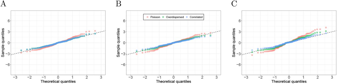
Exploration data analysis after fitting a standard Poisson model demonstrates that the daily data measurements are correlated (Supplementary Figure 8). Assuming independence, when in fact variables are correlated, leads to underestimates of the standard error of sums or averages. Cumulative excess mortality is the sum of excess deaths during a period of interest, therefore accounting for correlation allows our approach to better estimate the uncertainty of this quantity. To demonstrate this, we compared our model to a standard Poisson model and an over-dispersed Poisson model both assuming independent outcomes[14, 15, 16, 17]. As an illustrative example, we fit each of the three models to the Puerto Rico data for individuals 75 and over, and randomly selected 100 intervals of sizes L = 10, 50, and 100 days from periods with no events and computed the total number of deaths in each interval Sl = ∑t∊L Yt. We then used the fitted models to estimate the expected value Ê(Sl) and standard error and SÊ (Sl) and form a z-statistic Zl = [Sl − Ê (Sl)]/SÊ(Sl). The Central Limit Theorem predicts that, if the expected value and standard errors are estimated correctly, Zl is approximately normal with expected value 0 and standard error 1. We found that the Poisson and over-dispersed Poisson model underestimates the variance of this sum while modeling the correction improves our standard error estimates (Supplementary Figure 9).
3.6 An index based on relative proportion of specific causes of death
Limitations of our approaches for detecting and monitoring health crises in real-time are that it requires 1) complete death count data and 2) an estimate of population displacement. Note that incomplete death counts or underestimates of population displacement will result in an underestimate of the death rate. However, we if we know that a specific cause of death is associated with the event in question, we can construct an useful index that does not have these limitations. Specifically, if we redefine Yt as the number of deaths due to a specific cause at time t and Nt as the total number of recorded deaths at time t, then the estimate of f can be interpreted as the percent increase in the proportion of deaths due to that cause, even if the data is incomplete. The underlying cause of death for the Puerto Rico mortality data was coded using the tenth version of the International Classifications of Diseases (ICD10) codes[23]. Because deaths due to bacterial infections have been reported to increase after natural disasters in locations with poor public health infrastructure[24, 25], we defined an index based on ICD10 codes between A00 and A79 as bacterial infections. We found that deaths attributable to this cause were elevated after hurricane María in Puerto Rico (Figure 4A) pointing to the possibility that this index could be used in real-time to detect challenges to the health system. During the COVID-19 pandemic, if under-reporting is occurring, one would expect causes related to the respiratory system to increase. A similar index for respiratory diseases defined as ICD10 codes between J00 and J99 computed for the COVID-19 pandemic shows no anomalies (Figure 4B).
4 Discussion
We have introduced methods and software useful for estimating excess mortality from weekly or daily counts. The engine of our approach is a statistical model that accounts for long-term trends, seasonal effects, day of the week effects, and natural variation. An important contribution of this new approach is the improved uncertainty estimates permitted by modeling the correlation observed in the data. Another advance is the added flexibility that permits accounting for both direct and indirect effects.
We used the model to demonstrate that the indirect effects for Hurricanes Georges and María on Puerto Rico were like nothing seen in previous hurricanes in the United States. We also demonstrated that the 2014 Chikungunya epidemic resulted in substantial excess mortality in Puerto Rico. These results suggest a lack of robustness in Puerto Rico’s health system. We note that in New Orleans, shortly after Katrina, a $14.5 billion investment was made to construct stronger levees[26, 27, 28]. In contrast, after Hurricane Georges resulted in a similar excess mortality toll, as far as we know, no systematic effort was put in place to improve, for example, Puerto Rico’s electrical grid nor it’s data collection infrastructure. On the contrary, it appears that the grid continued to deteriorate during the 19 years between Georges and Maria. Furthermore, while Puerto Rico seems to have, up to now, dodged a bullet during the COVID-19 pandemic, its health system does not appear to be ready to withstand another shock to its fragile infrastructure. As an application of our method, we introduced an index that can be used in real-time to at least attempt to detect when there is a reason for concern.
Our analysis of CDC data demonstrated that by May 9, 2020, excess mortality was already above 100,000. We also performed a state-by-state analysis and found that over 58% of these deaths occurred in New York (37,070) and three of its neighbors: New Jersey (15,611), Pennsylvania (8,727), and Massachusetts (6,937). Note that Connecticut, the other neighboring state, was not included in the analysis due to missing data. However, it is important to note that the weekly death counts used in our analysis are adjusted for missing data by the CDC [12] and hence, the accuracy of our results depends on the accuracy of this adjustment.
Finally, we used our model to compare the effects of the pandemic in blacks and whites in Cook county, IL, and found a disturbing trend, with elderly blacks affected much more severely than their white counterparts. However, note that this analysis was not based on total mortality counts, but counts calculated from the Medical Examiner. Our conclusions assume that COVID-19 cases from whites and blacks are equally likely to be included in the Medical Examiner dataset.
When applying our methodology, there are several potential pitfalls and considerations to contemplate. First, one should be aware that the choice of spline knots can change the results. In general, we found that using 12 knots per-year was appropriate for exploring the data and detecting unknown periods of excess mortality, while six knots per year was appropriate to estimate indirect effects for hurricanes and outbreaks. However, we highly recommend viewing diagnostic plots that aid in determining if the model fits the data and sensitivity analysis to determine how much these choices affect final summaries. Our software provides tools that facilitate this. Second, we note that results depend on the population sizes Nt and that these are themselves estimates produced by government agencies. Third, we note that it is not always obvious if an increase in mortality should be classified as natural variability, several large εts, or an event for which f (t) > 0. This choice will often have to be guided by context and expertise rather than data. Finally, we point out that it is important to consider that our method does not permit the decoupling of estimated effects from different events during the same period. For example, the estimated effect for Hurricane María in Puerto Rico ran into the winter of 2017-2018 during which time some US states were affected by a particularly severe flu season.
Supplementary Material
1 Supplementary methods
Here we provide further details of our model and estimation approach. Further, we show that our model can also be applied to weekly data, show details on excess mortality calculations, and show results from a simulation study to validating our approach.
1.1 Model estimation
Our estimation procedure for model 1 involves three steps. We start by modeling the yearly trend α(t) with natural cubic splines with a knot every seven years. We model the seasonal effect s(t) with a harmonic model with 2 harmonics. Finally, w(t) represents seven parameters, one for each day of the week.
Natural disasters and outbreaks are rare, hence we assume that for the majority of time points f (t) is 0, which implies that
 and that, for example, for N = T/365 years of daily data we would have T data points to fit a model with at most N/7 + 7 + 4 + 1 parameters. For seven years of data this translates into 2,556 data points and 13 parameters. As a result, we can obtain highly precise estimates even in the presence of the extra dispersion introduced by ε. We therefore fit a Poisson Generalized Linear Model (GLM) to regions that we know do not include natural disasters or outbreaks and in the next step consider the MLE,
  , ŝ(t), and ŵ(t) as fixed.
In the second step we estimate Σ:
 where σ corresponds to the standard deviation associated with natural variability and ρh is the auto-correlation of two error terms that are h time units from each other. To do this we select a control contiguous region for which we know f (t) = 0. To estimate the σ2 and the autoregressive parameters we can use the law of total variance to note that the observed percent change from the mean
 has expected value and variance

Intuitively, these two components are the variance added by ε and the Poisson variability respectively. The above implies that if we define the transformation:
 we have an approximately normally distributed random variable with the same correlation structure as εt, which is what we want to estimate. We use the Yule-Walker equation approach to estimate the AR process parameters from the observed Zt. To estimate σ2 we use:
Using these estimates we can form an estimate  which we will consider known in the next step.
In the third step we treat  as known, assume f (t) can be modeled as a natural cubic spline, and use iteratively re-weighted least squares to obtain an estimate
  . To account for non-continuities due to direct effects from natural disasters we permit the spline to be discontinuous at the event day.
1.2 Approximation for uncorrelated data
Note that our model can be easily adapted to be fitted to weekly data. In this case there is no need to include weekday effect parameters w(t) and much less need for a correlation structure for the errors (Supplementary Figure 10).
1.3 Excess death estimates
We estimate cumulative excess deaths for any interval I = [a, b] by adding the excess deaths for each day in I:
We construct a 95% confidence interval using the fact that the sum  is approximately normally distributed, and if we define H as the hat matrix, we can compute the variace with:
  then
then
1.4 Simulation study
To assess our procedure we conducted a Monte Carlo simulation. We start by denoting: 1) an event day, t0, which may correspond to a hurricane landfall or peak-day of an epidemic, 2) an effect size, θ, that represents the percent change from expected mortality at event day, and 3) a period of effect, L, which constitutes the number of days with unusually high levels of mortality. Second, we use a normal distribution centered at t0 and scaled so that the value equals θ and that the standard deviation is equal to L/3 to estimate the true percent change in mortality, f(t). Then we compute  for t = 1, …, T, using the Puerto Rico mortality data with model (2) and generate rates
  . To generate the AR process, we first fit an AR model to our data and use the estimated coefficients to generate T auto-correlated errors ε1,…, ε T. We set the standard deviation of these errors to be σ = 0.05. Finally, we generate data
  . We generated three scenarios to mimic 1) a hurricane-like event where we expect mortality to increase rapidly and stay above normal levels for some time, 2) an epidemic-like event in which mortality increases slowly until reaching some plateau and then decreasing to normal levels, and 3) a time period of no event in which we expect our estimate of f(t) to be centered around 0. For each scenario we ran 100 simulations with t0 = September 21, 1998, θ = 0.55, and L = 150 days. Our implementation produces accurate and precise results for both f and Σ (Supplementary Figure 11).
2 Supplementary Figures

Estimated population displacement in Puerto Rico after Hurricane María.

Estimated components of the expected counts for six age groups in Puerto Rico. A) Death rate (deaths per 1,000 per year) trend components. B) Seasonal component for each age group as percentage increase or decrease from the average.

Estimated hurricane effects as percent increase over expected mortality for the six hurricanes. The solid line corresponds to percent change from expected mortality and the shaded region represents a 95% confidence interval.

Estimated effects as percent increase over expected mortality during the Chikungunya epidemic for different age groups. The solid line corresponds to percent change from expected mortality, the shaded region represents a 95% confidence interval, and points show observed percent change from expected mortality.

State-specific excess death estimates per 100,000 from March 1, 2020 to May 16, 2020, the period associated with the COVID-19 pandemic, plotted against the excess death estimates per 100,000 from December 10, 2017 to February 24, 2018, the period associated with the 2018 flu season. The identity line is represented in red and separates states in which the increase in mortality was higher during COVID-19 from those in which the increase in mortality was higher during the 2018 flu season.
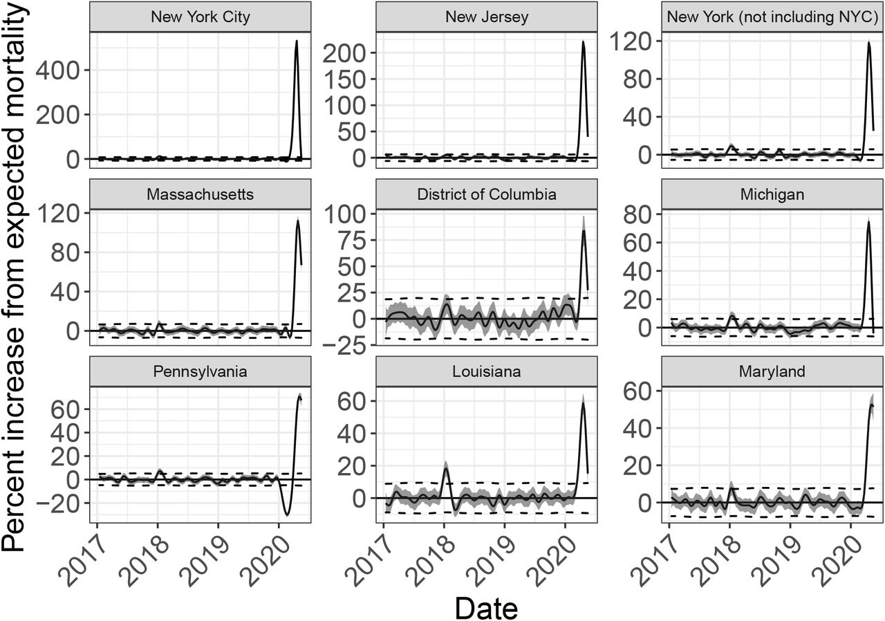
Estimated event effects as percent increase over expected mortality for New York City and 8 states in the United States with the largest percent increase in mortality rates during the COVID-19 pandemic. The solid line corresponds to percent change from expected mortality and the shaded region represents a 95% confidence interval. Note that no data was provided for Connecticut or North Carolina.

Estimated effect of the COVID-19 pandemic in Cook county, IL, as percent increase over expected mortality stratified by age groups. The solid line corresponds to percent change from expected mortality and the shaded region represents a 95% confidence interval.
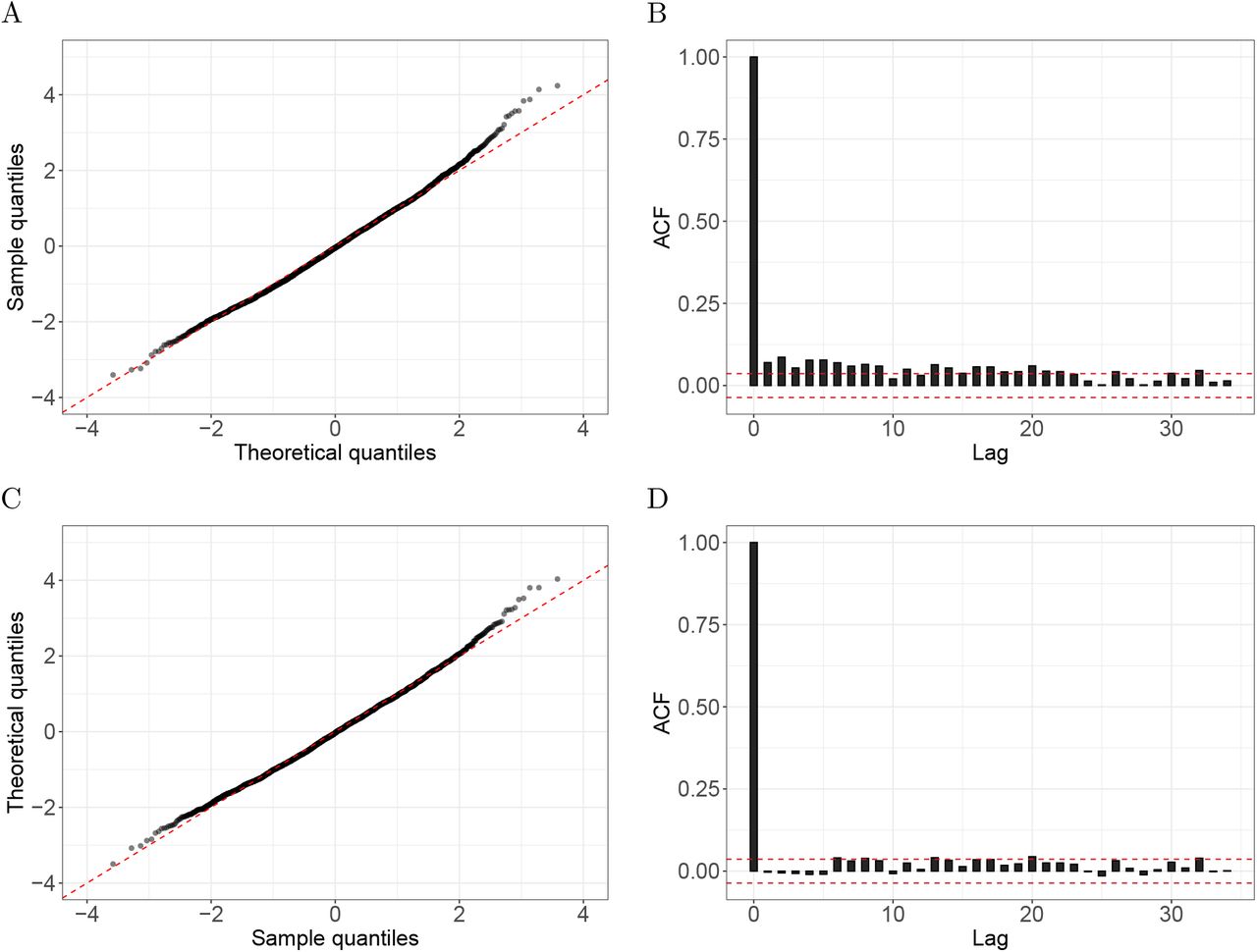
Evidence of correlated errors. A) A Poisson GLM was fitted to Puerto Rico daily death counts of individuals 75 years and over from an interval with no known natural disasters or outbreaks (Jan 1, 2006 to Dec 31, 2013). The plot shows the Pearson residuals quantiles versus theoretical quantiles from the normal distribution. One can see that the tail of the empirical data are larger than the theoretical values. B) The sample autocorrelation function for these Pearson residuals with the red-dash lines represent a 95% confidence interval centered at zero. C) As A) but for residuals after prewhitening based on an estimate of the covariance matrix. D) As B) but for the prewhittened residuals.

Accounting for correlation in the error structure improves uncertainty estimates. We fitted our model along with a Poisson and over-dispersed Poisson GLM to Puerto Rico data of individuals 75 years and over, and randomly picked 100 intervals of varying sizes to compute z-scores of total number of deaths. Each plot shows the Pearson residual quantiles versus theoretical quantiles from the standard normal distribution. A) Intervals of 10 days. B) Intervals of 50 days. C) Intervals of 100 days.

Accounting for correlation in the error structure of weekly data yields very similar uncertainty estimates to over-dispersed Poisson GLM. We fitted our model along with a Poisson and over-dispersed Poisson GLM to weekly Puerto Rico mortality data of individuals 75 years and over, and randomly picked 100 intervals of varying sizes to compute z-scores of total number of deaths. Each plot shows the Pearson residual quantiles versus theoretical quantiles from the standard normal distribution. A) Intervals of 1 week. B) Intervals of 7 weeks. C) Intervals of 14 weeks.

Simulation study. For all three scenarios, the event day (t0), the effect size (θ), and the period of effect (L) are September 21, 1998, 55%, and 150 days, respectively. For each scenario we ran 100 simulations. A) Percent increase in mortality from the average in the hypothetical scenario of a hurricane making landfall on September 21, 1998. The gray lines correspond to estimates from each simulation and the red line represents the true curve. B) Percent increase in mortality from the average in the hypothetical scenario of an epidemic with peak mortality on September 21, 1998. The gray lines correspond to estimates from each simulation and the red line represents the true curve. C) Percent change from expected mortality during a period with no event. D) Standard error of f(t) for estimates in A). The gray lines correspond to the standard error estimates for each simulation and the red line represents the true standard error, computed as the standard deviation of fitted values taken across simulations. E) As in D) but for estimates in B). F) As in D) but for estimates in C).
5 Acknowledgments
We thank Jose A. López Rodríguez from the Department of Health of Puerto Rico for diligently providing all the data we requested. We also thank Nicholas Kristof for making us aware of the CDC data. Further, we thank Florida, New Jersey, and Louisiana’s Department of Health for also providing the data we requested. Finally, we thank Canay Deniz, Andrea Samdahl, Lara Montini and Ilya Vasilenko from Teralytics for sharing their data and providing helpful explanations.
These findings and conclusion are those of the authors and do not necessarily represent the official position of the Puerto Rico, Florida, New Jersey, or Louisiana’s Department of Health, nor that of Teralytics.
References


Subject Area
Reviews and Context
0
Comment
0
TRIP Peer Reviews
0
Community Reviews
0
Automated Services
0
Blogs/Media
Author Videos