A novel COVID-19 epidemiological model with explicit susceptible and asymptomatic isolation compartments reveals unexpected consequences of timing social distancing

1 Introduction

Early 2020 saw the start of the coronavirus disease 2019 (COVID-19) pandemic, which is caused by severe acute respiratory syndrome coronavirus 2 (SARS-CoV-2). Current COVID-19 policy is being largely influenced by mathematical models [1, 2, 3, 4, 5, 6, 7, 8, 9]. Some of these are classic epidemiological ordinary differential equations (ODE) models. Such models are suitable for describing initial stages of an infection in a single city, as well as for describing late stages at which transportation effects are small in comparison to community spread. Besides being simpler to analyze mathematically, ODE models are also a component of more complex network simulations that incorporate interacting populations linked by transportation networks as well as social, school, and workplace hubs. The work described here is in the spirit of the former, ODE models.

We have developed and analyzed a variation of the classic epidemiological SIR model which incorporates separate “compartments” for “socially distanced” healthy and asymptomatic (but infected) populations, as well as for infected (symptomatic) populations. There have been many models proposed in the literature to deal with “quarantined” populations, see for example [10, 11], but, to the best of our knowledge, no models in which susceptible populations are split into non-distanced and distanced sub-classes in such a way that the rates of flow between these are viewed as control variables. Indeed, key to our model are parameters that reflect the rate at which individuals become “socially distant” and the rate at which individuals return to the “non-distanced” category. As examples, the latter might represent a “frustration” with isolation rules, or a personal need to reduce the economic impact of social distancing. The former can be in principle manipulated by government intervention, through the strength of persuasion, and law enforcement.

How do outcomes depend on such interventions? How does one trade-off various types of other interventions (for example vaccination, which would affect transmissibility, or curfew rules) against each other? Our modeling work aims to provide a framework to rigorously formulate and answer such questions.

We will view the rate at which individuals respond to mandates as a control variable, and analyze the impact of different control policies on the course of an epidemic. A novel aspect of our model lies in the distinction that we make between rate control and the decrease in contacts between infected and susceptible individuals due to distancing. We call this latter reduction in transmission the contact rescaling factor (CoRF). One can interpret the CoRF value as reflecting the effectiveness of social distancing. This number is a function of the stringency of rules (stay at home except for shopping and emergencies, wash hands frequently, wear masks, stay 6 ft. apart, etc.). Some authors consider tuning what we call the CoRF as the control “knob” used by authorities, e.g. [12, 13, 14, 15, 16]. Our focus is, instead, on rate control, which has not been sufficiently explored. Indeed, the objective of our model is to make it possible to formally consider rate control. In future work, we will study the combination of rate and CoRF control.

In particular, we used our model to answer questions about the dynamics of the disease, and about the value of the basic reproduction number, R₀, which characterizes the initial rise in infections. We rigorously demonstrate, without simulations, that at sufficiently early stages of the pandemic when there is little immunity in the population, no amount of social distancing will result in R₀ < 1. While it is easy to interpret this as a hopeless situation, what this actually says is that an initially headline-grabbing infection will begin to move through the population. However, as time progresses, we show that social distancing can indeed have the desired effect of pushing R₀ to a value less than 1 by accelerating the approach to herd immunity,

This conclusion about the impact of social distancing at different stages on the pandemic is dependent on the parameter choices made in the model. As many of these parameters are still uncertain, we also explored how R₀ depends on a combination of a single model parameter and the social distancing parameter. One major unknown about COVID-19 is the fraction of individuals who get infected but never develop symptoms. We find that R₀ is very sensitive to this symptomatic fraction, demonstrating the importance of getting a confident measurement on this value before quantitative model predictions can be trusted.

Another major unknown is how infective asymptomatic individuals are. We find that if asymptomatics are not very contagious, and if infected individuals automatically self-isolate, then R₀ is not greatly influenced by social distancing measures. However, if asymptomatics are sufficiently infective, there is a much stronger impact of social distancing on R₀. That said, this conclusion depends on the assumption that social distancing reduces the transmission rate of the disease, through what we called the contact rescaling factor (CoRF). Therefore, varying this parameter allows us to quantify how the nature of social distancing measures impacts R₀. If this parameter is very small, meaning one significantly downscales their contacts (that is, the stay-at-home directives are extreme), very rapid implementation of social distancing is not required. On the other hand, if the directives are not as severe and CoRF is larger (meaning the number of contacts is scaled down less significantly), social distancing will not result in R₀ < 1 and we can still expect disease spread despite social distancing.

We also used our model to explore how the timing of social distancing influences the spread of the disease through a population. One of the most striking predictions is that a slight delay in establishing social distancing guidelines (on the order of up to a month with our parameters) does not appreciably influence the course of the disease. We were initially surprised by this result, which means that authorities can take some time to plan for guidelines. However, the fact that R₀ > 1, meaning that there will be an initial exponential increase in infections no matter the strength of the guidelines, is consistent with this prediction. Notably, we also find the existence of what we term a critical implementation delay (CID), about a month in our model, where even a few days delay in implementation beyond that critical time can have highly adverse consequences. One might call this phenomenon it is OK to take some time to plan, but then implement immediately”.

Related to timing, there has been interest in periodically relaxing distancing guidelines to allow for limited economic activity. For example, businesses may be allowed to operate normally for one week, while the ensuing week is restricted to remote operation (or being fully closed, if remote work is not feasible). This two week “periodic” schedule is then continued either for a fixed period of time, or indefinitely (e.g. the discovery of a vaccine, evidence that sufficient herd immunity has been obtained, etc.) Using our model with estimated parameters, we simulate such schedules for a variety of periods, ranging from days to months of sanctioned activity. Our results are quite counter-intuitive, and suggest that there might be a pulsing period that significantly inhibits the infection dynamics (a 28 day “on/off” schedule with our parameters). However, this schedule is exceptionally sensitive to parameter values and timing, so that extreme caution must be taken when designing guidelines that fully relax social distancing, even temporarily. Furthermore, for some strategies near the optimal 28-day cycle, a subsequent increase in infected individuals may occur after an initial flattening. Thus, even if a region observes a short-term improvement, the worst may still be yet to come.

Other forms of relaxation relate to gradual easing, as opposed to periods of “normal activity.” Of course, the rate of easing (e.g. how many people are allowed in a grocery store or in an office) is of great interest, both economically and psychologically. We numerically investigate how the rate of easing social distancing guidelines affects outbreak dynamics, and show that relaxing too quickly will only delay, but not suppress, the peak magnitude of symptomatic individuals. However, a more gradual relaxation schedule will both delay onset and “flatten the curve,” while producing a largely immune population after a fixed policy window (again, assuming recovery corresponds to immunity, which is still an open question as of this writing). Hence the rate of relaxation is an important factor in mitigating the severity of the current pandemic. Similarly, the rate of relaxation during flattening is important to prevent a “second wave” of infected individuals. As governments develop and implement plans to ease social distancing, carefully considering the rate of relaxation is extremely important from a policy perspective, so that countries and states do not undo the benefits of their strict distancing policies by lifting guidelines too rapidly. For example, in our model, a very rapid relaxation schedule results in a second wave with a larger peak symptomatic proportion than originally experienced (over 21%, compared to original peak of 17.6%). However, relaxing more gradually once the peak has been obtained prevents a second outbreak, and allows a sustainable approach to herd immunity.

We close this introduction with this quote:

“I have skepticism about models [of COVID-19], and they are only as good as the assumptions you put into them, but they are not completely misleading. They are telling you something that is a reality, that when you have mitigation that is containing something, and unless it is down, in the right direction, and you pull back prematurely, you are going to get a rebound of cases.”

Dr. Anthony Fauci, Director, National Institute of Allergy and Infectious Diseases, United States; on CNN, 05 May 2020

It bears emphasizing: ours is one model, with one set of assumptions. We do not in any way believe that the quantitative predictions of our (or of any other) model of COVID-19 can be accurate, as so much is still unknown about this disease. However, as in the statistician George Box’s aphorism “All models are wrong, but some are useful”, the correct question is not if the model is “true” but rather if it is “illuminating and useful.”

2 Models

The SIR model proposed by W.O. Kermack and A.G. McKendrick in 1927 [17] has been applied in many ways over the last century to study infectious diseases, and recently has been extended to study COVID-19. For example, a recent model for COVID-19, called the SIDARTHE model [12], partitions individuals as susceptibles, asymptomatic and undetected infected, asymptomatic detected, symptomatic undetected, symptomatic detected, detected with life-threatening symptoms, recovered, and deceased. There are also several papers that deal with timing of interventions as well as periodic strategies to prevent the spread of epidemics, modeled through periodic vaccination [18] or through the periodic or other switching of the infectivity parameter β in SIR and related models [12, 14, 15, 16].

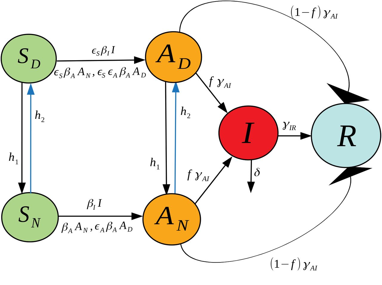
In this work we propose a different extension of the SIR model, one that includes socially distanced (labeled with a D sub-index) and non-socially distanced (labeled with an N sub-index) classes for susceptible (S_D and S_N), asymptomatic (A_D and A_N), and symptomatic (I_D and I_N) individuals. Class R refers to “Recovered” who are presumed to have developed at least temporary immunity. More details about the interpretation of each variable together with the meaning of the parameter symbols used in this model can be found at Table 1. Next, we explain the dynamics of our model (please refer to Fig. 1 for a graphical explanation):

1. A socially distanced susceptible individual (S_D) may become infected with rate:

   • ∊_Sβ_AA_N when in contact with a non-socially distanced asymptomatic individual. Here, β_A is the transmission rate between an asymptomatic non-socially distanced individual and a non-socially distanced susceptible; and the term ∊_S accounts for the reduction of infectivity by socially distancing the susceptible. We call ∊_S a contact rescaling factor (CoRF).

   • ∊_S∊_Aβ_AA_D when in contact with a socially distanced asymptomatic individual. The term ∊_S∊_A refers to the reduction of infectivity by socially distancing both the susceptible and the asymptomatic individuals.

   • ∊_Sβ_II_N when in contact with a non-socially distanced symptomatic individual. The term β_I denotes the transmission rate between non-socially distant symptomatic and non-socially distanced susceptible individuals.

   • ∊_S∊_Iβ_II_Dwhen in contact with a non-socially distanced symptomatic individual. The term ∊_S∊_I denotes the reduction of infectivity by socially distancing both the susceptible and the symptomatic individuals. We expect that socially distanced symptomatic individuals are still capable of transmitting infections, be it through contact with hospital personnel or caregivers.

2. Similarly, a non-socially distanced susceptible individual (S_N) may become infected with rate:

   • β_AA_N when in contact with a non-socially distanced asymptomatic individual.

   • ∊_Aβ_AA_D when in contact with a socially distanced asymptomatic individual.

   • β_II_N when in contact with a non-socially distanced symptomatic individual.

   • ∊_Iβ_II_D when in contact with a socially distanced symptomatic individual.

3. If a susceptible individual that has been social distancing (an individual in class S_D) gets infected, they will continue social distancing (will transfer to class A_D); and a non-social distanced individual will continue non-social distancing right after getting infected (it will transition from the S_N to the A_N class).

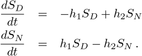
4. Susceptible individuals transition from social distancing to non-social distancing behavior with rate h₁. Likewise for asymptomatic individuals.

5. Susceptible individuals transition from non-social distancing to social distancing behavior with rate h₂. Likewise for asymptomatic individuals.

6. After the incubation period, an asymptomatic individual may or may not become symptomatic. Thus, it may transition from the asymptomatic class into the symptomatic class, or directly to the removed class. The symbol f represents the fraction of the asymptomatic individuals that transition into the symptomatic class. Thus (1 - f) is the fraction of individuals who are asymptomatic and transition directly to the recovered group.

7. The transition rate out of asymptomatic, γ_AI, is independent of whether one was socially distancing or not.

8. A fraction p of non-socially distanced asymptomatic start social distancing after becoming symptomatic. Thus, (1 - p) is the fraction of non-socially distanced asymptomatic individuals that remain non-social distancing after becoming symptomatic.

9. A social distancing asymptomatic that becomes symptomatic remains socially distancing (transfers from A_D into I_D).

10. If an individual becomes symptomatic, they will either recover (transfer to the R class with rate γ_IR) or die with rate δ.

11. Recovery assumes that the individual will acquire temporary immunity.

12. Recovered individuals lose immunity at a rate ρ.

13. A fraction q of recovered individuals who lost immunity remain socially distanced, and a fraction (1 - q) will stop social distancing.

• Download figure
• Open in new tab

Figure 1:

Illustration of the seven compartment SIR model in eqns. (1)-(7)

The differential equation system representing this seven-compartment model is as follows:

Although very little is known about immunity in regards to COVID-19, it is known that for other types of coronaviruses such as the severe acute respiratory syndrome (SARS) antibodies are maintained for an average of two years [19, 20, 21].

At present, pharmaceutical companies around the world are working to acquire a vaccine for COVID-19, and it is hoped that one will be widely deployed in less than two years. For this reason, we are currently interested in understanding the dynamics that will occur during the waiting period for a vaccine. It seems reasonable then, under the assumption that a recovered individual may acquire immunity for an average period of two years, to start by studying the simplified model where immunity is not temporary. Further, given the widespread understanding of the contagious nature of SARS-CoV-2, it is also reasonable to assume that symptomatic individuals self-isolate.

2.1 A simplified version (A six compartment SIR Model)

In this simplified model we assume permanent immunity for the recovered class, and that all symptomatics (I_N and I_D) can be merged into just one class I (see Fig. 2). The differential equation system representing this model is given below:

• Download figure
• Open in new tab

Figure 2:

Illustration of the six compartment SIR model in eqns. (8)-(13).

2.2 Parameter estimation from currently available data

We first note that the variables in our model system (8)-(13) should be interpreted in terms of fractions of the population, and not as absolute population numbers. Of course, a direct translation is possible by fitting to a region of interest, and multiplying by a total population size at the time of disease outbreak. Note that since the initial conditions are all non-negative and satisfy then all variables remain in the interval [0,1] for future times t > 0, and can hence be interpreted as a fraction of the initial population. Note that if δ > 0 (a strictly positive death rate) and (14) is satisfied, the total population fraction N defined by will satisfy for all t > 0. In fact, the difference 1 − N(t) measures the fraction of deaths of the initial population by time t. Births are ignored, since we consider time-scales on the order of 1 year, and newborns are not significant contributors to the susceptible populations.

It is easy to verify (see Appendix C) that all the infective populations, A_N (t), A_D (t), and I(t) converge to zero as t →∞. One contribution of this work is to make the distinction between rate control and decrease in contacts due to social distancing. Hence, we need to explicitly define rate control (h₁ and h₂) in our model. To this end, recall that h₁ is interpreted as a socializing rate, while h₂ is a controlled level of social distancing. Intuitively, we expect that increasing social distancing guidelines will at the same time inhibit individuals from socializing. That is, h₁ and h₂ are not independent, but are rather inversely correlated to one another. To make this mathematically precise, we define

That is, increasing distancing mandates (h₂) at the same time decreases the rate at which individuals socialize (h₁). Other functional relationships are possible, but for the remainder of this work we fix h₁ as in eqn. (18). Furthermore, we fix so that

It is difficult to estimate such rates directly, as they correspond to sociological responses to unprecedented self-isolation guidelines. However, our rationale is as follows. Consider first a policy such that h₂ = 1 per day, which implies that (interpreting the ODE system as the expected value of the corresponding Poisson process) that the average time to socially distance is

Assuming that the population is initially non-distanced, so that S_N (0) ≈ 1, S_D (0) ≈ 0, and ignoring the infection dynamics over a period of 1 day, we have the estimate

In the above, we ignored transitions from S_D into S_N, as S_D is assumed small. Hence, after 1 day, approximately 63% of the population socially distances. Equation (20) then yields , so that of the (assumed small) socially distanced

That is, about 9% of the population disobeys the distancing mandate per day. Similarly, when h₂ = 0, i.e. there are no social distancing directives, eqn. (20) yields h₁ = 1, so that i.e. about 63% of the population re-socializes in 1 day; others may be too scared, or simply not prone to leave their house every day. The above reasoning seems at least reasonable to the authors. Of course, the focus on the subsequent analysis will not be on precise predictions, but rather general phenomenon, which are robust to parameter values. This should be considered for the remainder of this section (and the remainder of the work) as we discuss other estimates.

We can also interpret h₁ and h₂ in terms of the equilibrium fractions of socially distanced individuals. Indeed, in the absence of any infection (assuming no recovery has yet taken place), we have the equilibrium fractions of S_N and S_D are given by

If as above, h₂ = 1, then , and we have that

Hence, in the long-term, with very strict distancing guidelines, approximately 92% of the susceptible population will distance, while 8% do not. This also seems reasonable with very strict mandates, as of course some jobs remain essential and hence not all workers can become isolated (nurses, doctors, grocery workers, first responders, etc.).

Recall that fγ_AI is the transition rate from the asymptomatic (but infected) populations A_D and A_N. Again interpreting as the expected value of a Poisson process, we can relate fγ_AI to the expected time until asymptomatic individuals shows symptoms

That is, fγ_AI is inversely proportional the incubation period of the disease. There are different estimates of this incubation period. The original analysis based on 88 confirmed cases in Chinese provinces outside Wuhan, using data on known travel to and from Wuhan, gave an estimate of 6.4 days [22]. Later estimates of community spread have been closer to 5.1 days, with a 95% confidence interval of 4.1 to 7.0 days [23, 24]. We picked the number 〈t_A〉 = 6.2 in this interval, to account for about a day earlier exposure that would account for an adjustment for travel, but our results do not change substantially if a slightly smaller value is used. Thus at our chosen value of ƒ, this yields

We fix this value in the remainder of the work. Note that all rates will be measured in days.

In a similar manner, we estimate the parameter γ_IR, the transition rate from infected to recovered. The February 2020 joint WHO-China report [25] found an average recovery time of 2 weeks at the time of the onset of symptoms for mild cases, and 3 – 6 weeks for severe cases. In our model, we do not distinguish between the types of symptomatic individuals, and hence we roughly estimate an average 3 week recovery period. Hence

The parameter ƒ represents the fraction of SARS-CoV-2 infections that become symptomatic. Current reports suggest that this parameter is highly variable, with analyses on different data sets yielding between 20% - 95% of positive tested cases being symptomatic (so that ƒ ∈ [0.2,0.95]) [26, 27, 28, 29, 30, 31, 32, 33, 34, 35]. We use the Diamond Princess cruise ship data from Yokohama Japan, which had 634 positive cases. In [26], the authors estimate the asymptomatic proportion of positive cases to be 17.9%, and so we fix ƒ as

Finally, we can estimate δ, the disease mortality rate, on the fraction of reported deaths with respect to the total disease numbers. Using global data reported on the John Hopkins dashboard [36] on 03/29/2020, there were a total of 33876 deaths and 717656 reported cases, so that

Using the above value of γ_IR in (36), we thus have that

The remaining parameters are β_A, β_I, ∊_A, and ∊_S. For simplicity, we assume that the effect of social distancing the susceptible and asymptomatic individuals is symmetric, so that

β_A and ∊_A will be calibrated to reported R₀ values in Section 3.1.

3 Results

3.1 Basic Reproduction Number, R₀

A central subject in the analysis of epidemiological models concerns the stability of a “disease free steady state” (abbreviated DFSS from now on), in which all infective populations are set to zero. Stability of the DFSS means that small perturbations of the DFSS, that is to say, the introduction of a small number of infectives into the population, results in exponential convergence back to the DFSS. In other words, the infection does not take hold in the population. Mathematically, this means that the linearization at the DFSS is described by a matrix in which all eigenvalues have negative real part (a “Hurwitz matrix”). Conversely, if the DFSS is unstable, then the infection will initially expand exponentially. It is important to realize, however, a very subtle and often misunderstood fact. Instability of the DFSS does not necessarily imply that the infection will keep increasing forever. Linearized analysis is only local, and says nothing about behavior over long time horizons, because nonlinear effects can dominate once the system is away from the DFSS; indeed, we will show that we find this phenomenon in our model (provided that social distancing directives are introduced).

A fundamental and beautiful mathematical result is that the DFSS is exponentially stable if and only if the basic reproduction number R₀ is less than one. Intuitively, R₀ is the average number of new infections that is caused by a typical individual during the period that this individual is infective. Mathematically, R₀ is defined as the dominant eigenvalue of a certain positive matrix, called the next generation matrix [38, 39]. We briefly explain this method in Appendix A, and therein derive that for our six-compartment SIR model in eqns. 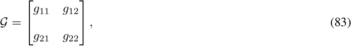(8)-(13): where g_ij represents the (i, j) −entry of the next generation matrix G evaluated at the DFSS. As we derive in Appendix A: where represents the value of S_N at the DFSS.

We begin here by studying the value of R₀ under various scenarios of disease progression. We distinguish these scenarios by a number we call R^* that gives the percent of the population that has “recovered” from the disease.¹ Herein we assume all recovered have developed immunity, though that assumption could easily be removed. One can interpret R^* = 0 as the very earliest stage of the pandemic, when there are no recovered individuals in the population. On the other extreme, R^* = 1 indicates every individual has recovered. Because we are assuming all recovereds stay recovered, increasing values of R^* correspond to increasing values of time.

In Fig. 3, we show how R₀ (as predicted by our model) changes as a function of the fraction of recovered R^* and the rate of social distancing h₂. We observe that at sufficiently early stages of the pandemic (R^* < 0.35), R₀ > 1 no matter how strong the rate of social distancing. (The contact rescaling factor CoRF is kept constant, as explained in the Introduction). While it is easy to interpret this as saying controlling the disease is hopeless, this is not the case. As discussed above, instability of the DFSS does not characterize global temporal behavior. It does tell us that an “overshoot” and headline-grabbing infection will initially take hold. Thus, social distancing directives will initially appear to have failed in their intended effect. But, as time goes on and more individuals in the population become recovered, social distancing can eventually result in R₀ < 1, which would result in the epidemic dying out exponentially.

Of course, giving a precise meaning to “small” is impossible from linearized analysis alone, and requires a deeper understanding of local/global analysis, by appeal for example to Lyapunov functions (see for instance [40]). Nonetheless, we found out that this argument is in excellent agreement with simulations, and hence we use formulas for R₀ as a function of R^* (and of other parameters in the model as well) to understand how sensitive R₀ is to different social distancing rates, the point in time when such directives are introduced (as quantified by R^*), and other parameters. Also note that, even when R₀ > 1, social distancing can still “flatten the curve”, as we show in Section 3.2. This means that the peak infection levels will be lower, which reduces the stress on the healthcare system.

Fig. 3(b) indicates that, once the rate of social distancing is sufficiently large, increasing the rate has no measurable impact on R₀. To explore this eventual insensitivity to h₂ further, we note that the limit of R₀ as h₂ → ∞ to can be written as , where and, specifically for our parameters in Table 2:

View this table:

• View inline
• View popup
• Download powerpoint

Table 2:

A list of estimated parameters values to be used in our simulations.

• Download figure
• Open in new tab

Figure 3:

Basic reproduction number as a function of the social distancing rate parameter h₂ and R^*, the fraction of the population that is immune. All other parameters as in Table 2.

The formulas follow from the explicit calculation of R₀ given in Appendix A. We show in Fig. 4 plots of R₀ as a function of h₂ for R^* =0 (on the interval h₂ ∊ [0,1], where we get already close to the asymptotic value 1.4953), as well as its derivative and its differential sensitivity, defined intuitively as and formally as 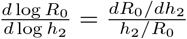. The fact that this sensitivity rapidly approaches zero means that after a threshold rate of social distancing, small relative changes in the rate of social distancing have essentially no effect on relative changes in R₀.

Mathematically, it is interesting that the derivative of R₀ (and also the sensitivity) does not always have the same sign, in other words can change sign. This is necessary because , but this second derivative cannot stay negative since R₀ is bounded below. Taken together, these plots further confirm that expediting the timing to put social distancing into effect beyond a certain threshold does not result in significant changes to R₀.

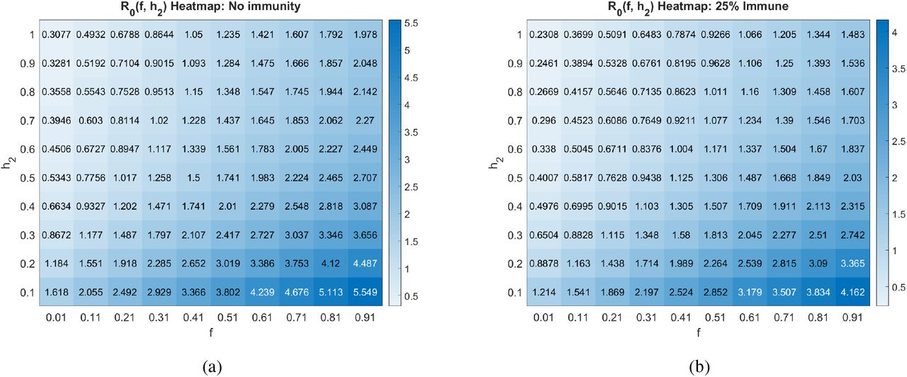
We proceed by exploring the sensitivity of R₀ to various combinations of parameters, all including the social distancing rate h₂. The first parameter we consider is ƒ, which determines the fraction of asymptomatic individuals that progress to having disease symptoms. As Fig. 5 indicates, the value of R₀ is extremely sensitive to the fraction of individuals that develop symptoms, whether we are at an earlier (R^* = 0) or later (R^* = 0.25) stage of the pandemic. In particular, a larger likelihood of transitioning from asymptomatic to symptomatic dramatically increases R₀. This occurs because both asymptomatics and symptomatics spread the disease, so spending time in both A and I means the individual has more time to spread the disease than if an individual transitions directly from the asymptomatic pool to the recovered pool. Current data makes it quite difficult to know what ƒ is for SARS-CoV-2. Data from a cruise ship [26], which we used to calibrate our model, found ƒ ≈ 0.821. However, more recent data out of Italy suggests ƒ may be closer to 0.57 [35]. Without any social distancing directives, this reduction in ƒ would reduce R₀ from 6 to 4.5 at our baseline parameters. Further, the recognition that there may be different strains of SARS-CoV-2 could mean that ƒ varies depending on the dominant strain in a region [41].

• Download figure
• Open in new tab

Figure 4:

Plots of R₀, derivative dR₀/dh₂, and differential sensitivity 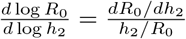, all as functions of h₂ at R^* = 0. Different ranges picked for clarity. R₀ converges to ≈ 1.4953 as h₂ → ∞, while dR₀/dh₂ and differential sensitivity all converge to zero.

• Download figure
• Open in new tab

Figure 5:

Basic reproduction number as a function of the social distancing rate parameter h₂ and fraction of individuals who become symptomatic (ƒ) at different pandemic stages. All other parameters as in Table 2.

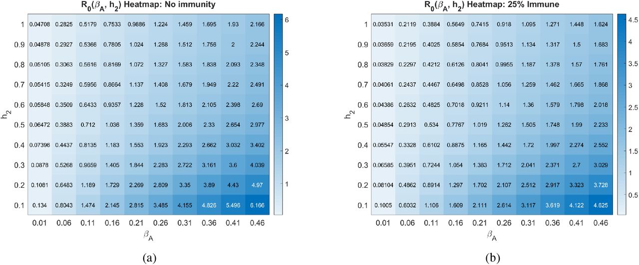
Another uncertainty surrounding COVID-19 is how infectious the asymptomatic individuals are, which we call β_A in our model. In Fig. 6, we explore how the contagion level of the asymptomatics influences R₀ under varying rates of social distancing. We observe that if asymptomatics are not very contagious (β_A is small), then R₀ is not very sensitive to social distancing directives as measured by h₂ (R₀-clines are almost vertical). This can be explained by our assumption that symptomatic individuals are assumed to socially distance themselves, and therefore have minimal interaction in our model with susceptibles. When this is the case, the disease is mainly spread by non-socially distanced asymptomatics. And, if the transmission rate from these individuals is small, socially distancing the asymptomatics and susceptibles has little impact on the progression of the disease. If, on the other hand, β_A is sufficiently large, than asymptomatics can fairly readily seread the disease, and we see a much strong impact of social distancing on R₀ (R₀-clines get much less steep as β_A increases).

• Download figure
• Open in new tab

Figure 6:

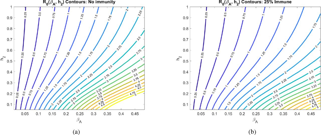
Basic reproduction number as a function of the social distancing rate parameter h₂ and infectivity rate of asymptomatics β_A at different pandemic stages. All other parameters as in Table 2.

Another major assumption of our model is that social distancing reduces the transmission rate of the disease by a factor called the contact rescaling factor (CoRF). We formulate our model so that socially distancing the susceptibles and the asymptomatics (note, infectives are assumed to be socially distanced) are described by different CoRF values of ∊_S and ∊_A, respectively. However, in all calculations and simulations, we assume that the extent that social distancing reduces the transmission rate is the same independent of whether an individual is susceptible, asymptomatic, or infected. That is, we take ∊:= ∊_S = ∊_A. The value of the CoRF ∊ is another way to measure social-distancing directives. While h₂ describes rate of social distancing, ∊ describes the severity of the measures. While not realistic for a disease like COVID-19, if socially distancing meant an individual was exposed to nobody else, the contact rescaling factor ∊ would be 0. Intuitively, and as we quantitatively demonstrate in Fig. 7, at very small e, the rate of social-distancing h₂ is less important. Social-distancing is still needed for R₀ < 1, but R₀ drops below 1 at the fairly small rate of h₂ = 0.2 when there are no recovered in the population, and at h₂ = 0.12 when 25% of the population has recovered.

• Download figure
• Open in new tab

Figure 7:

Basic reproduction number as a function of the social rate distancing parameter h₂ and the contact rescaling factor (CoRF) ∊ at different pandemic stages. CoRF measures the impact of social distancing on infectivity rate. All other parameters as in Table 2.

Increasing the CoRF ∊ can be thought of as increasing the number of contacts socially-distanced individuals have. With all other parameters fixed as specified in Table 2, we see that social distance rate h₂ can only result in an R₀ < 1 at the early stages of the pandemic if the CoRF ∊ is less than 0.25. Beyond this value, even socially-distanced individuals have too many contacts, and R₀ > 1. Intuitively, we see that R₀ quickly increases as the CoRF increases. This shows that, even if individuals act very quick to socially distance (there is a large h₂), if they have too many contacts while social distancing, social distancing will not be sufficient to drive R₀ < 1.

3.2 Time-varying social distancing (h₂(t))

We now investigate how dynamic social distancing protocols affect the spread of the epidemic in the model introduced in Section 2.1.

3.2.1 No distancing dynamics

We begin with the predicted outbreak dynamics in the case of no implementd social distancing. As discussed in Section 3.1, with parameters estimated from data, we expect so that we expect the disease to spread rapidly throughout the population. No social distancing implies that

Initial conditions consist of all susceptible individuals socially non-distanced, no population immunity, and a small number of symptomatic individuals (100 in 10 million). More precisely,

Of course, in reality it is likely that a number of asymptomatic people also exist in the population at this time (t = 0), but for simplicity we ignore them. Note that I(0) was taken to be consistent (as an order of magnitude) with the reported cases in New York City (NYC) before a state of emergency was declared (89 cases on March 7, with a total NYC population of approximately 8.4 million). These will be the initial conditions used throughout the remainder of the manuscript, as we compare intervention strategies based on responses to the above infection data at time day t = 0.

The results of simulating the model in eqns. (8)-(13) for 180 days are provided in Figure 8. This will serve as a baseline for the severity of the outbreak in a “worst-case scenario.” Social distancing strategies will be compared to these worst-case figures, some of which we highlight below:

1. The symptomatic infected population (I) reaches a peak value of 41.81% at any one given time.

2. The time to this peak is approximately 51 days.

3. The model predicts that a peak of 60% of the total infected population (symptomatic and asymptomatic) will occur at day 45.

4. By day 100, 90% of the population will be recovered (assuming recovereds do not lose immunity).

5. Almost 4% of the population will die during the outbreak (3.92%).

6. Compartments S_D and A_D never comprise any percentage of the population. This is because of the initial conditions, and because no distancing guidelines have been issued in this “worst-case scenario”.

• Download figure
• Open in new tab

Figure 8:

Population responses in the absence of treatment. Here h₂(t) = 0, i.e. no social distancing has been implemented. We simulated the model introduced in Section 2.1 for 180 days. Note that the infected symptomatic population (I, solid red curve) comprises about 42% of the population by day 51.

3.2.2 Delayed response

We first investigate disease dynamics in response to delayed social distancing protocols. We assume that h₂(t) takes the following form:

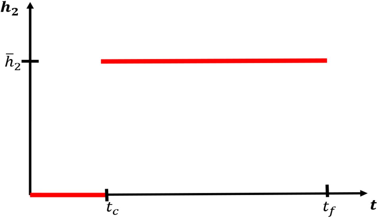
That is, we assume that social distancing does not occur until an implementation time t_c, after which h₂(t) is kept at a constant value . For a visualization, see Figure 9.

• Download figure
• Open in new tab

Figure 9:

Social distancing control as a function of the delay t_c. Functional form for h₂ used in Figure 11. See also eqn. (54).

Since many policies are implemented in a 48 hour window, we set

Fixing all other parameters as in Table 2, we simulate the model for a range of policy activation days t_c; results are shown in Figure 10. Here we observe an apparent “flattening of the curve,” if the distancing was enacted quickly enough. That is, if polices were enacted too late, social distancing has little effect on the course of the outbreak; the response to a delay of 50 days is nearly identical to one with no distancing imposed. This is hardly surprising, since if a society waits too long to start socially distancing, the disease will have already spread through much of the population. However, if the delay is short enough (i.e. the response quick enough), we see a significant reduction in the peak of the infected population (17% for a t_c = 10 days, compared to the worst-case of 42%). Furthermore, there seems to be a critical “window of opportunity” for commencing social distancing: the difference between waiting 30 and 40 days is quite striking (peak of 20% in the former, up to 35% in the latter). Notice that this window of opportunity ends at a time (about 30 days) that is much earlier than the time at which infections would have peaked in the absence of control measures (about 51 days). We think of (roughly) 30 days as a critical implementation delay (CID).

• Download figure
• Open in new tab

Figure 10:

Population response for a treatment window of 180 days with varying start time t_c of social-distancing protocol (see Figure 9). Left panel denotes the symptomatic (I) temporal response; right indicates the recovered percentages for each policy. Red curves correspond to no social distancing (see Figure 8). Note that a delay of 50 days is hardly discernible from no social distancing, while a significant response transition occurs for delays longer than 30 days.

We investigate this further by plotting both the peak symptomatic population and the time to this peak in Figure 11, where social distancing is begun at t = t_c days, for t_c = 0,1,2,…, 60. This provides a quantification of what we saw in Figure 10: if the delay is relatively small or large, the response (measured as peak infected percentage) is robust to the delay. However, there is a critical window about which a “bifurcation” occurs. For our parameters, the bifurcation value appears to be approximately 1 month. In that first month, if social distancing is begun, the outbreak will be sharply inhibited. However, near this critical value, delaying even a few extra days could drastically increase the total number of symptomatic individuals; for example, waiting 34 days yields a peak of 23% symptomatic, while waiting an extra week increases the peak to over 36%. Thus we see that policies will be effective in a certain window, and that it is critical to implement them within that window. Indeed, delaying even by a few days outside of that window could severely increase the total number of infections.

• Download figure
• Open in new tab

Figure 11:

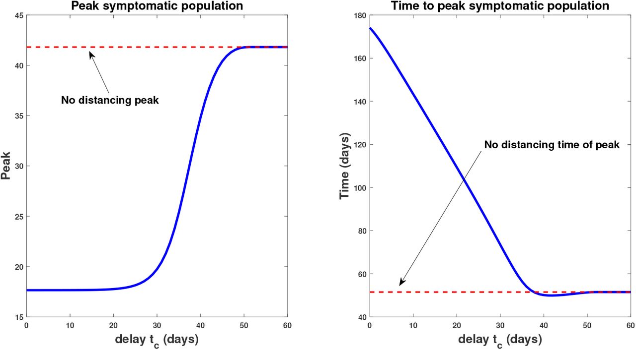
Peak infected population percentage (left) and time to this peak (right) when social distancing is delayed. Here the horizontal axis represents the delay (from time t = 0), i.e. the value t_c in (54). The dotted red line denotes the corresponding values when no social distancing is enacted (Section 3.2.1). Note the rapid increase in peak symptomatic population beginning around 30 days, which we term a critical implementation delay (CID).

We also note that the time to peak number of symptomatic individuals (right panel, Figure 11) increases the sooner the distancing procedure is implemented. This is intuitive, and combined with the previous result says that the more quickly social distancing is enacted, the longer you will have to deal with a smaller number of sick individuals. However, the number of sick individuals is relatively constant up until a certain time delay, where once passed, there will be many more (over twice) the number of sick people in the population at its worst moment. Hence, on the policy level, it is okay to take some time to plan a strategy, but once decided, it must be implemented quickly and efficiently.

3.2.3 Periodic relaxation

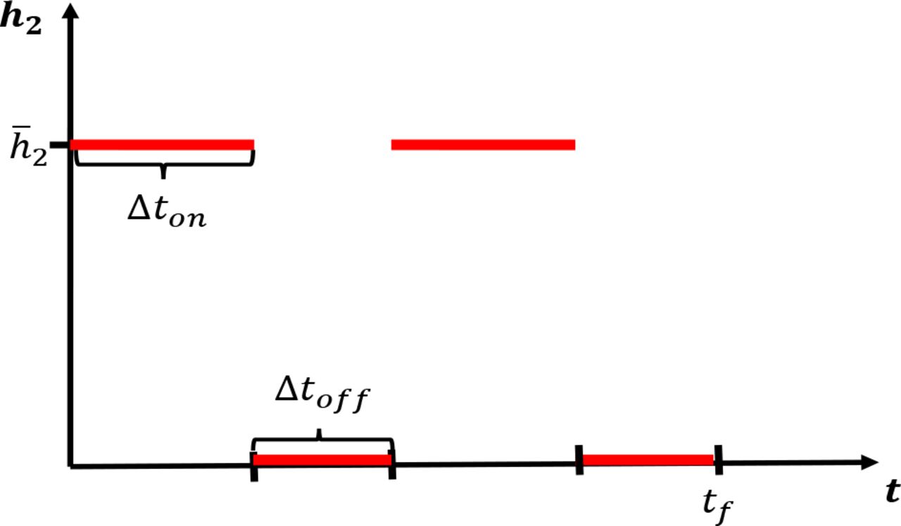
We next investigate the effects of periodically relaxing social distancing protocols. Consider a protocol where social distancing measures are implemented for a fixed time window ∆t_on followed by a relaxation ∆t_off. The above is then repeated until a final time t_f is reached. We envision a situation where the population is allowed to interact normally for (say) one week, but must then isolate for the following week. Such policies may lessen the economic and psychological impact of extended complete isolation by allowing limited windows in which individuals may work, socialize, etc. For a visualization of a simplified version of such a policy, see Figure 12. Note that we consider total relaxation (h₂ = 0) during ∆t_off, but of course this could be adjusted; here we consider the simplest possible periodic (i.e. metronomic) policy.

• Download figure
• Open in new tab

Figure 12:

Pulsing of socially distancing protocol. Social distancing is enacted for a time length of ∆t_on days, followed by a full relaxation for ∆t_off days. This schedule is then repeated until a time window t_ƒ has been reached.

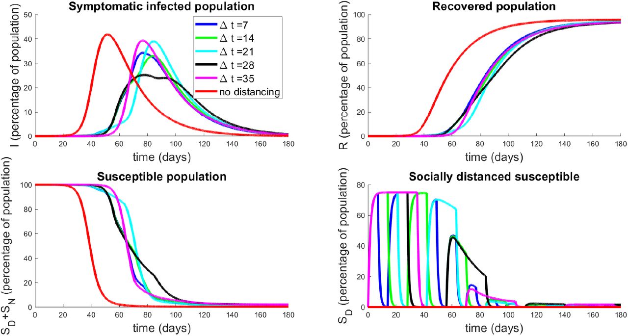
In Figure 13, we investigate the dynamical response to several schedules with varying number of weeks of distancing. We assume that the lengths of activation and relaxation are equal, so that

• Download figure
• Open in new tab

Figure 13:

Population response to strategies based on periodic relaxation of social distancing; see Figure 12. Top left panel denotes temporal dynamics of symptomatic population (I) for pulsing strategies with ∆t_on = ∆t_off = ∆t. Non-socially distanced dynamics (red curves) are provided for comparison. Top right panel is recovered population in time, and bottom panels are total susceptible individuals (left) and socially-distanced susceptible individuals (right). Initial conditions are described in Section 3.2.1.

Note that this restriction allows a relatively unbiased comparison between distancing protocols, since all will have distancing enacted for the same total amount of time. There is a slight discrepancy based on t_f, since the schedules may end at different points of their respective cycles, but this effect is minimal. Hence we conclude that each schedule will have approximately the same economic impact, and hence in the following we only examine the disease response. Note that we fix as in Section 3.2.2.

The results presented in Figure 13 are quite surprising and non-intuitive. Note that they all have delayed the onset of the peak of the epidemic by a similar length of time (all around 75 - 85 days, whereas the epidemic would have originally peaked at around 51 days). However, the degree to which the peak has been suppressed is different among the relaxation schedules. It appears that high frequency pulsing (small ∆t) does better than some extended strategies (compare ∆t = 7 to ∆t = 21, 35), but worse than others (compare ∆t = 7 to ∆t = 14 or 28). This seems to indicate that there is some optimal pulsing period. Furthermore, the curve for ∆t = 28 is quite interesting; we see a significant reduction in peak population infection (25%, compared to 42%) together with an extended “flattening of the curve”, which does not appear in the others. We also note that all strategies end with similar recovery rates (all above 94%, top right panel, Figure 13).

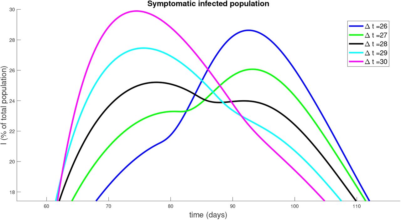
To understand the behavior near ∆t = 28, we simulate a series of strategies with ∆t near this value, and observe how the symptomatic response varies. Results are provided in Figure 14 for ∆t = 26,27,28,29,30. Note that the peak infected proportion appears to interact with a concavity change near ∆t = 28, and this interaction causes a significant decrease in the peak together with an extended “flattening” period. However, it is relatively sensitive to the timing, so that a slight error in timing (or a slight variation in parameters) will cause a large increase in peak infected numbers. Another interesting property is apparent in the curve with ∆t = 27: we see an initial flattening of infectivity, followed by an increase in the number of symptomatic individuals. Hence for some strategies, the progression may yet worsen even after an apparent downward trend. Phenomenologically, we see a “bifurcation” between two “unimodal” behaviors in time (earlier vs. later peak) that happens through a “bimodal” (two maximal) time behavior (centered around for a period of around 55 days corresponding to 27.5 days of distancing and 27.5 days of non-distancing).

• Download figure
• Open in new tab

Figure 14:

Similar to Figure 13, but for policies with ∆t near 28 days.

We also globally investigate the response of different pulsing frequencies (different ∆t) on the critical infection measures of peak symptomatic individuals and the corresponding time of this peak. A simulation of pulsing strategies with periods ranging from ∆t =1 day to ∆t = 90 days is presented in Figure 15. The left panel denotes a clearly non-monotone global response to different periodic relaxation schedules. Furthermore, we observe a global minimum near ∆t = 28 days, as discussed previously. Note also the sensitivity to the period: ∆ = 28 days yields a peak of only 24%, while a slightly faster relaxation schedule of ∆ = 20 days produces a peak of nearly 40%. Hence, designing such strategies is inherently risky, and should be done only when parameter values are precisely known.

• Download figure
• Open in new tab

Figure 15:

Response of infection dynamics to periodic relaxation for a range of frequencies. Policy period is assumed for 180 days. Left panel denotes peak symptomatic population (percentage) at any one time. Right panel is the corresponding time (in days) when this peak occurs. Initial conditions are described in Section 3.2.1.

3.2.4 Relaxing social distancing

We next investigate the rate at which social distancing policies are eased after a fixed period of time. Such control strategies may be important to prevent a second wave of infection arising soon after policies are relaxed. In this section, we model the effects of a controlled relaxation on outbreak dynamics. The control we consider takes the form of a linear decrease in regulations after a fixed isolation period (t₁ days). The rate of decrease is determined by an end time t_e, after which social distancing is no longer encouraged. Thus, a larger value of t_e corresponds to a slower easing of restrictions. For a visualization, see Figure 16. We fix to capture current conditions.

• Download figure
• Open in new tab

Figure 16:

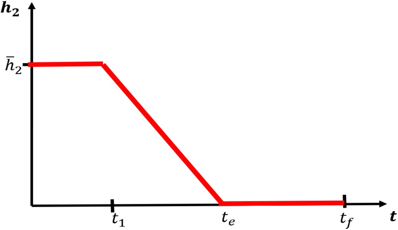
Relaxing social distancing measures after an initial period of strict regulations for t₁ days. Rate is decreased linearly from h₂ at day t₁ to 0 at day t_e. After day t_e, no distancing regulations are in place.

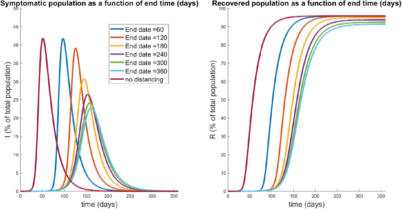
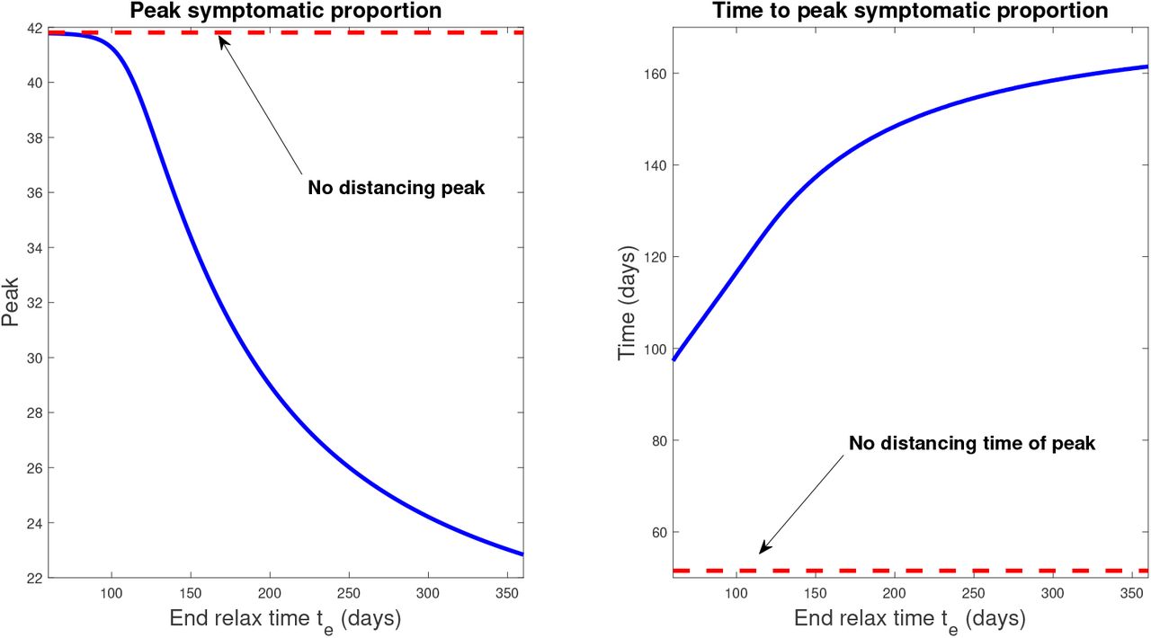
Results of simulation data for select relaxation rates appear in Fig. 17, while a global characterization is provided by Fig. 18. Note that t_e = 60 days corresponds to immediately turning social distancing off (a step, i.e. infinite slope), while t_e = 360 corresponds to a relaxation rate of slope 0.0017. Results indicate that gradual relaxation does have a significant effect on “flattening the curve” in that it results in a lower peak infected population over a larger time interval (compare t_e = 60 to t_e = 360 in Fig. 17). Fig. 18 further supports this claim, as we compute little variation in the peak for small relaxation times (corresponding to more quickly ending protocols), but that a substantial decrease in symptomatic burden is obtained as t_e is increased. Indeed, for a gradual relaxation over a one year period (360 days), we see a peak symptomatic population of only 22%, which is down significantly from immediate re-openings after 60 days (42%). Note that the latter schedule does result in any significant peak mitigation when compared to the policy of no social distancing: it merely delays the same peak by approximately 46 days. Hence it seems crucially important to gradually relax social distancing guidelines, as gradually as is economically feasible, to help mitigate the outbreak.

• Download figure
• Open in new tab

Figure 17:

Symptomatic (left) and recovered (right) populations for policies which relax social distancing at a rate determined (inversely) by t_e, the day at which distancing policies are completely removed. The response for no social distancing implemented is included for reference (red curves). Note that t_e = 60 corresponds to immediate relaxation, and has a similar peak to the non-distanced curve. However, gradual relaxation protocols appear to both decrease the peak number of symptomatic individuals, while also spreading out their distribution.

• Download figure
• Open in new tab

Figure 18:

Response of infection dynamics to different relaxation rates after 60 days of social distancing. Policy period is assumed for 360 days. Left panel denotes peak symptomatic population (percentage) at any one time. Right panel is the corresponding time (in days) when this peak occurs. Initial conditions are described in Section 3.2.1.

We also see that, as in Section 3.2.3, all strategies result in a significant fraction of the population being immune by t_f = 360 days. In other words, under the assumption that infection confers immunity that lasts at least a year, herd immunity has been largely achieved in all protocols.

3.2.5 Relaxation and a second outbreak

In Section 3.2.4, we saw that the rate of relaxation of social distancing was related to the overall peak symptomatic population: relax too quickly, and the peak is delayed but not inhibited, but gradually lift polices and this peak is both reduced and delayed to a substantial degree. (Figs. 17 and 18). In that analysis, we assumed a fixed distancing period of 60 days, after which relaxation protocols are implemented. In reality however, policies are not designed utilizing artificial timelines, but instead rely on measured data relating to the epidemiology of the outbreak. A question many states and countries now face is the following: given that we observe a “flattening of the curve” (e.g. a plateau of new reported cases), how should relaxation be implemented? In this section, we use our model to address this question.

Consider an initial outbreak as discussed in Section 3.2.1 (specifically initial conditions in eqn. (53)), after which a strict social distancing protocol is enforced. Mathematically, this means that

As in the previous sections, we fix which implies that

The above policies are applied until the outbreak, here measured as the growth of the symptomatic population, dissipates. That is, we apply the above until a time t_d such that

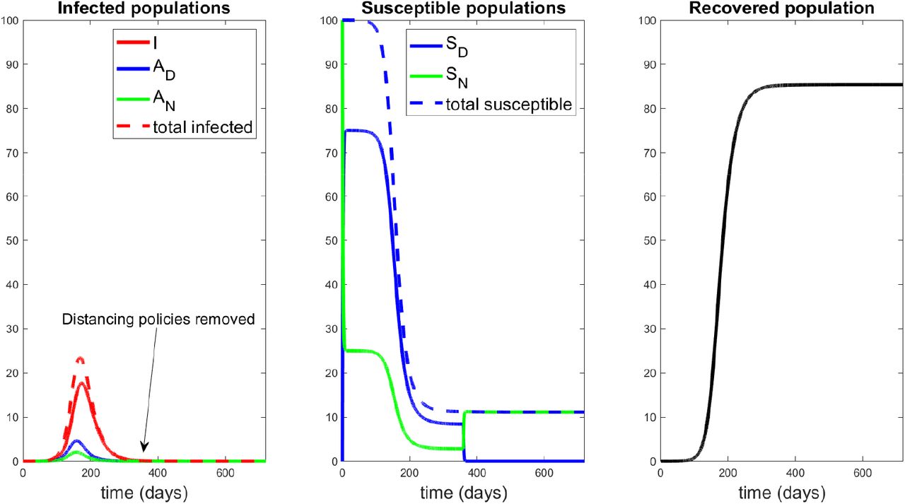
At time t_d, from a policy perspective, it appears that the “worst is over,” and hence we should begin the process of relaxing social distancing. Indeed, if we continued the process for 360 days (well beyond the peak t_d), our model and parameters suggest a response as seen in Fig. 19. Hence, with current available measures, the best that can be accomplished is the response provided in Figure 19, and thus it is natural to study the question of relaxation once the peak is reached (about 17.6% symptomatic at day t_d = 174). Note that social distancing guidelines were ceased at day 360, and no second outbreak was subsequently observed. This agrees with our calculations of R₀ in Section 3.1 (in particular Figure 3 (a)), which yields R₀ < 1 for h₂ = 0, R^* = R(360) = 85%. Hence we expect no further outbreak after 360 days of social distancing, due to the large recovered population (an assumption in the model, but by no means experimentally verified; indeed our results will be quite different if re-infection is allowed).

• Download figure
• Open in new tab

Figure 19:

Response to 360 days of social distancing, with h₂ as in eqn. (59) for t ∊ [0,360] days, after which h₂(t) = 0. Note the peak of the symptomatic population is approximately 17.6% of the population, occurring at around day 174. Even after social distancing measures are stopped, no subsequent outbreak occurs.

We thus consider a relaxation policy similar to that shown in Fig. 16, with t_d taking the role of t₁, and investigate the response to different relaxation policies (different t_e). From Fig.19, we see that t_d is given by

The dynamical response of our model to selected relaxation rates appears in Fig. 20, while a more global characterization is provided in Figure 21. Note in the left panel of Figure 20, all protocols have the same response until time t = t_d (black curve); this is because social distancing is identically enforced for 0 ≤ t ≤ t_d. After t_d, we see a different infection response based upon the rate at which distancing policies are relaxed. Note that if the rate of relaxation is too large (t_e = 175, 185 days in Fig. 20), we see a second wave of infections, larger than the original peak. For example, if social distancing policies are concluded by day 175 (a very small relaxation period, since relaxing begun on day 174), we see a second peak of symptomatic individuals of over 21% of the population by day 192; compare this with the original peak of 17.6%. However, if relaxation is relatively slow (for example, t_e = 250 days), we see no second wave of infection. Hence in designing policy, we must carefully consider the manner in which social distancing policies are removed; if it is too fast, then we risk undoing the work achieved in the first t_d = 174 days.

• Download figure
• Open in new tab

Figure 20:

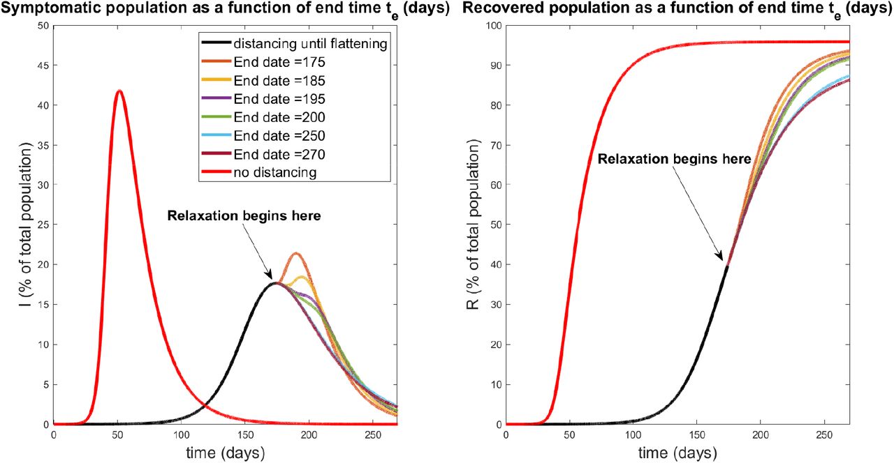
Relaxation during flattening. Symptomatic (left) and recovered (right) populations for policies which relax social distancing at a rate determined (inversely) by t_e, the day at which distancing policies are completely removed. The response for no social distancing implemented is included for reference (red curves). All curves besides the red curve are identical for the first t_d = 174 days of treatment, when social distancing is implemented with per day. Note that a second wave occurs for relaxation protocols that end quickly (t_e = 175,185 days). However, if relaxation is slow enough (larger t_e), a second wave of infection is completely mitigated. All simulations are taken over 270 days.

In Fig. 21, we provide a plot of the peak of the second wave as a function of both the full relaxation time (left) and the relaxation rate (right). Note that the rate is the speed (magnitude) of the relaxation schedule, and corresponds to the absolute value of the slope in Fig. 16. The time t_e and rate are thus related via

• Download figure
• Open in new tab

Figure 21:

Magnitudes of second wave of symptomatic individuals (percentage of total population) as a function of end time t_e (left) and rate (right). Note that t_e and relaxation rate are inversely proportional; see eqn. (63). A second peak of 0 indicates that no second outbreak occurred fr the corresponding relaxation schedule. Red curve denotes first wave peak, which occurs for all schedules at day t_d = 174. All simulations are taken over 270 days.

• Download figure
• Open in new tab

Figure 22:

Basic reproduction number as a function of social distancing parameter h₂ and R^*, the fraction of the population that is immune. All other parameters as in Table 2.

• Download figure
• Open in new tab

Figure 23:

Basic reproduction number as a function of the social distancing rate parameter h₂ and fraction of individuals who become symptomatic (ƒ) at different pandemic stages. All other parameters as in Table 2.

• Download figure
• Open in new tab

Figure 24:

Basic reproduction number as a function of the social distancing rate parameter h₂ and infectivity rate of asymptomatics β_A at different pandemic stages. All other parameters as in Table 2.

• Download figure
• Open in new tab

Figure 25:

Basic reproduction number as a function of the social distancing rate parameter h₂ and the contact rescaling factor (CoRF) ∊ at different pandemic stages. CoRF measures the impact of social distancing on infectivity rate. All other parameters as in Table 2.

If no second peak occurs, we set the corresponding value to 0. Hence we compute a critical relaxation rate r_c, such that if social distancing is relaxed faster than r_c, a second outbreak will occur (right panel of Figure 21). However, if distancing restrictions are eased slowly enough (i.e. slower than r_c), a second peak never occurs, and herd immunity is achieved after 270 days (again, assuming it exists). For our parameters, we find that this critical rate is

Hence we may provide an estimate to the degree to which social distancing may be relaxed. Of course, this value depends critically on parameter values and other assumptions which remain (as of writing) unknown. Indeed, the main conclusion should not be the exact value given in eqn. (64), but rather the phenomenon that the “speed” of relaxation has significant consequences for subsequent outbreaks, which we believe is robust with respect to parameter values.

4 Discussion & Conclusion

In this work, we have introduced a novel epidemiological model of the COVID-19 pandemic which incorporates explicit social distancing via separate compartments for susceptible and asymptomatic (but infectious) individuals. We believe that this is the first model which characterizes social distancing protocols as rates of flow between these compartments, with the rates determined by guidelines implemented by regional governmental intervention. In particular, we view these rates as controls, and one of our primary focuses of study is disease response (measured by peak symptomatic proportion) to different mandated social distancing controls.

Our major contributions are described below:

1. In model formulation, we decouple the rate of social distancing (h₂) with the decrease in contact due to social distancing (∊_S, ∊_A, ∊_I). The latter we term the contact rescaling factor (CoRF), which should be interpreted as an effectiveness of social distancing. Hence we explicitly account for both the rate at which individuals distance, and how effective distancing is as a means of suppressing viral transmission.

2. The basic reproduction number, R₀, is explicitly calculated for our model system. For parameters obtained from data, we show that no amount of distancing will result in an R₀ < 1, i.e. that there will always be an initial outbreak of the COVID-19 pandemic. However, the situation is not hopeless, as social distancing policies are able to push R₀ < 1 as the disease spreads throughout the population.

3. R₀ is very sensitive to the fraction of infective individuals that are asymptomatic, and to the infectivity of these asymptomatic individuals. Hence understanding this population (through, for example, widespread testing) is critical for making informed policy decisions.

4. There is a critical time to implement social distancing guidelines (what we label the critical intervention delay (CID)), after which social distancing will have little effect on mitigating the outbreak. Surprising, the CID occurs well before the peak symptomatic proportion would have originally appeared under non-distanced protocols (CID is approximately 30 days for our parameter values, while non-distanced peak occurs at about 51 days).

5. Periodic relaxation strategies, where normal behavior is allowed for certain periods of time, can significantly reduce the symptomatic burden. However, such scheduling is not robust, and small errors (either in timing, or via parameter estimation) may have catastrophic repercussions.

6. Gradual relaxation can substantially improve the overall symptomatic response, but the rate of relaxation is important to prevent a “second wave” of virus outbreak. Prolonged relaxation and relaxation at flattening can significantly “flatten the curve.”

As noted throughout the manuscript, exact predictions rely on estimated parameter values, which currently vary widely throughout the literature. On the other hand, we believe that the qualitative phenomenon observed are robust, and should be considered during policy design.

Future work will involve a more systematic control analysis involving both the rate of social distancing (h₂) and the stringency of distancing (CoRF, i.e. ∊ terms). Ideally, we would like to minimize the peak of the symptomatic population (I) while simultaneously maximizing the time to reach this peak; we view such an objective as a precise quantification of “flattening the curve.” This must be done with distancing constraints imposed, to reflect the fact that a certain percentage of the population must remain active to maintain a functional society (healthcare workers, food supply, emergency responders, etc.). Using optimal control and feedback laws, our model can help inform policy makers as they make difficult decisions about how to adapt to the ongoing pandemic.

Author Contributions

Conception and design: All authors.

Development of methodology: All authors.

Analysis and interpretation of data: All authors.

Writing, review and/or revision of manuscript: All authors.

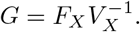
A The Basic Reproduction Number R₀

The next generation matrix algorithm, proposed by Diekmann at. al. in 1990 [38], is a technique used to calculate the basic reproduction number R₀. We explain it briefly, for more details see [39, 42].

Here are the steps to compute the next generation matrix G:

1. Let X = {x₁, x₂,…, x_n} represent the n infected host compartments, and Y = {y₁, y₂, …, y_m} represent the m other host compartments.

2. Write your ODE system as: where F_i represents the rate at which new infectives enter compartment i, and V_i represents the transfer of individuals out of and into the i-th compartment.

3. Let F_X and V_X represent the Jacobian matrices evaluated at the DFSS of the vector fields respectively.

4. The next generation matrix G is defined by

   G is a non-negative matrix with an eigenvalue which is real, positive, and strictly greater than all the others. This largest eigenvalue is R₀.

A.1 R₀ for the six-compartment SIR model (equations (8)-(13))

We compute the basic reproduction number R₀ of the six-compartment SIR model with the Next Generation Matrix Algorithm [38, 39, 42].

Let

Thus, 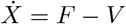where F_X and V_X denote the Jacobian matrices of f and V respectively (i have not evaluated at the DFSS yet. I will do it once I find G, there is no much simplification evaluating at this step); and

Let g_ij represents the (i, j)-entry of the next generation matrix G. Notice that the g_ij are already evaluated at DFSS, where we must satisfy the equation 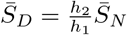. Thus, where represents the value of S_N at DFSS. Here, G has characteristic polynomial: with roots (eigenvalues of G):

Therefore, λ₃ is the basic reproduction number, R₀.

A.1.1 Conditions for R₀ < 1. The case h₂ =0 for the six-compartment SIR model

If h₂, the rate of social distancing, is equals to zero (which implies ). The basic reproduction number reduces to:

In other words,

For R₀ to be less than 1 we must satisfy the equation: or equivalently,

A.1.2 Conditions for R₀ < 1. The general case for the six-compartment SIR model

Let , and consider the polynomial where b and c are the trace and determinant of the matrix respectively.

Remark 1.

• 

• 2. The discriminant .

• 3. The eigenvalues of are:

  where λ₁ < λ₂ and λ₂ > 0. 4. Let

• 4. Let where

  Thus, .

• 5. At disease-free equilibrium the following equations are satisfied: which gives the relation

  Therefore,

• 6. From equation (91), it follows that R₀ < 1 if and only if

• 7. For , equation (92) is equivalent to

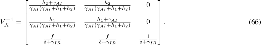
A.2 R₀ for the seven-compartment SIR model (equations (1)-(7))

Let

Thus, and where F_X and V_X denote the Jacobian matrices of F and V respectively; and 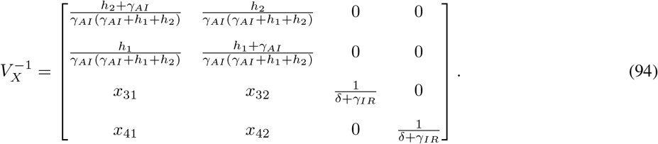with

Let g_ij represents the (i, j)—entry of the next generation matrix G. Notice that the g_ij are already evaluated at DFSS, where we must satisfy the equation 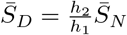. Thus,

Thus, is the characteristic polynomial of G with roots:

Therefore, λ₃ is the basic reproduction number, R₀.

B Heatmaps Corresponding to Contour Plots of R₀

C Convergence of infectives to zero

It is a routine exercise to show that, in our model, I(t) → 0 as t → ∞, and similarly for A_N (t) and A_D (t). Indeed, consider the total population fraction N defined by N:= S_D + S_N + A_D + A_N + I + R and observe that dN/dt = δI ≤ 0. The function N is continuously differentiable. The LaSalle Invariance Principle [43] implies that all solutions converge to an invariant set Ω included in dN/dt = 0, meaning in particular that all solutions have I(t) → 0, as claimed. Furthermore, the equation dI/dt = fγ_AI(A_D + A_N) − δI − γ_IRI when restricted to Ω says that 0 = fγ_AI(A_D(t) + A_N(t)), which means that, in this set to which all solutions converge, both A_D and A_N are identically zero.

As dR/dt = 0 on this set Ω, R(t) converges to a limit r (which is in general nonzero). The equations for susceptibles

Thus S_D and S_N equilibrate to constant values under the constraint that S_D + S_N = n − r, where n = lim_t→∞ N(t), i.e. .