
Abstract
Establishing how many people have already been infected by SARS-CoV-2 is an urgent priority for controlling the COVID-19 pandemic. Patchy virological testing has hampered interpretation of confirmed case counts, and unknown rates of asymptomatic and mild infections make it challenging to develop evidence-based public health policies. Serological tests that identify past infection can be used to estimate cumulative incidence, but the relative accuracy and robustness of various sampling strategies has been unclear. Here, we used a flexible framework that integrates uncertainty from test characteristics, sample size, and heterogeneity in seroprevalence across tested subpopulations to compare estimates from sampling schemes. Using the same framework and making the assumption that serological positivity indicates immune protection, we propagated these estimates and uncertainty through dynamical models to assess the uncertainty in the epidemiological parameters needed to evaluate public health interventions. We examined the relative accuracy of convenience samples versus structured surveys to estimate population seroprevalence, and found that sampling schemes informed by demographics and contact networks outperform uniform sampling. The framework can be adapted to optimize the design of serological surveys given particular test characteristics and capacity, population demography, sampling strategy, and modeling approach, and can be tailored to support decision-making around introducing or removing interventions.
Introduction
Serological testing is a critical component of the response to COVID-19 as well as to future epidemics. Assessment of population seropositivity, a measure of the prevalence of individuals who have been infected in the past and developed antibodies to the virus, can address gaps in knowledge of the cumulative disease incidence. This is particularly important given inadequate viral diagnostic testing and incomplete understanding of the rates of mild and asymptomatic infections (1). In this context, serological surveillance has the potential to provide information about the true number of infections, allowing for robust estimates of case and infection fatality rates and for the parameterization of epidemiological models to evaluate the possible impacts of specific interventions and thus guide public health decision-making.
The proportion of the population that has been infected by, and recovered from, the coronavirus causing COVID-19 will be a critical measure to inform policies on a population level, including when and how social distancing interventions can be relaxed. Individual serological testing may allow low-risk individuals to return to work, school, or college, contingent on the immune protection afforded by a measurable antibody response. At a population level, however, methods are urgently needed to design and interpret serological data based on testing of sub-populations, including convenience samples that are likely to be tested first, to reliably estimate population seroprevalence.
Three sources of uncertainty complicate efforts to learn population seroprevalence from sub-sampling. First, tests may have imperfect sensitivity and specificity; estimates for COVID-19 tests on the market as of April 2020 reported specificity between 95% and 100% and sensitivity between 62% and 97% (Supplementary Table S1). Second, the population sampled will likely not be a representative random sample, particularly in the first rounds of testing, when there is urgency to test using convenience samples and potentially limited serological testing capacity. Third, there is uncertainty inherent to any model-based forecast which uses the empirical estimation of seroprevalence, regardless of the quality of the test, in part because of the uncertain relationship between seropositivity and immunity (2).
A clear evidence-based guide to aid the design of serological studies is critical to policy makers and public health officials both for estimation of seroprevalence and for forward-looking modeling efforts, particularly if serological positivity reflects immune protection. To address this need, we developed a framework that can be used to design and interpret serological studies, with applicability to SARS-CoV-2. Starting with results from a serological survey of a given size and age stratification, the framework incorporates the test’s sensitivity and specificity and enables estimates of population seroprevalence that include uncertainty. These estimates can then be used in models of disease spread to calculate the effective reproductive number Reff, the transmission potential of SARS-CoV-2 under partial immunity, to forecast disease dynamics, and to assess the impact of candidate public health and clinical interventions. Similarly, starting with a pre-specified tolerance for uncertainty in seroprevalence estimates, the framework can be used to define the sample size needed. This framework can be used in conjunction with any model, including ODE models (3, 4), agent-based simulations (5), or network simulations (6), and can be used to estimate Reff or to simulate transmission dynamics.
Results
The overall framework is described in Fig. 1, showing that the workflow can be used in two directions. In the forward direction, starting from serological data, one can estimate seroprevalence. While valuable on its own, seroprevalence can also be used as the input to an appropriate model to update forecasts or estimate the impacts of interventions. In the reverse direction, sample sizes can be calculated to yield estimates with a desired level of uncertainty and efficient sampling strategies can be developed based on prospective modeling tasks.

Test sensitivity/specificity, sampling bias, and true seroprevalence influence the accuracy and robustness of estimates
To integrate uncertainty arising from test sensitivity and specificity, we produced a Bayesian posterior distribution of seroprevalence that accommodates uncertainty associated with a finite sample size (Fig. 1; green annotations). We denote the posterior probability that the true population serology is equal to θ, given test outcome data X and test sensitivity and specificity characteristics, as Pr(θ | X). Because sample size and outcomes are included in X, and because test sensitivity and specificity are included in the calculations, this posterior distribution over θ appropriately handles uncertainty (see Methods).
To illustrate the use of these calculations in practice, we first simulated serological data from populations with seroprevalence rates ranging from 1% to 50% using the reported sensitivity (93%) and specificity (97.5%) of a test approved for sale in the EU (Supplementary Table S1), and with the number of samples ranging from 100 to 5000. Next, we constructed Bayesian posterior estimates of seroprevalence (see Methods), finding that, when seroprevalence is 10% or lower, around 1000 samples are necessary to estimate seroprevalence to within two percentage points (Fig. 2). Tests with other characteristics required around 1000 tests (93.8% sensitivity, 97.5% specificity; Supplementary Fig. S1A) and 750 tests (97.2% sensitivity and 100% specificity; Supplementary Fig. S1B) to achieve the same uncertainty levels, relative to the minimum of around 650 tests for a theoretical test with perfect sensitivity and specificity (Supplementary Fig. S1C).

Uncertainty, represented by the width of 90% credible intervals, is presented as ± seroprevalence percentage points in (A) a heatmap and (B) for selected seroprevalence values, based on a serological test with 93% sensitivity and 97.5% specificity (Supplementary Fig. S1 depicts results for other sensitivity and specificity values). 5000 samples are sufficient to estimate any seroprevalence to within a worst-case tolerance of ± 1.3 percentage points, even with the imperfect test studied. Each point or pixel is averaged over 250 stochastic draws from the specified seroprevalence with the indicated sensitivity and specificity.
Sampling frameworks for seropositivity estimates are likely to be non-random and constrained to subpopulations. Therefore, although general estimates were most uncertain when true seropositivity was near 50%, the number of samples was low, and/or test sensitivity/specificity were low (Fig. 2 and Supplementary Fig. S1), another source of statistical uncertainty comes from the potentially uneven distribution of samples across a population with variation in true positivity. To extrapolate seropositivity from a sample of a particular subpopulation, we specified a Bayesian hierarchical model by introducing a common prior distribution on subpopulation-specific seropositivities θi (see Methods). In effect, this allowed seropositivity estimates from individual subpopulations to inform each other while still taking into account subpopulation-specific testing outcomes.
Convenience sampling (testing blood samples that were obtained for another purpose and are readily available) will often be the easiest and quickest data collection method (7). Two examples of such convenience samples are newborn heel stick dried blood spots, which contain maternal antibodies and thus reflect maternal exposure, and serum from blood donors. Sampling may also be designed to represent a broader range of the population, such as random uniform sampling across age groups, sampling informed by population demographics, or sampling in relation to expectations about contribution to transmission, for example based on an age-structured contact matrix (8–10). We termed this latter sampling scheme ‘model and demographics informed’ sampling.
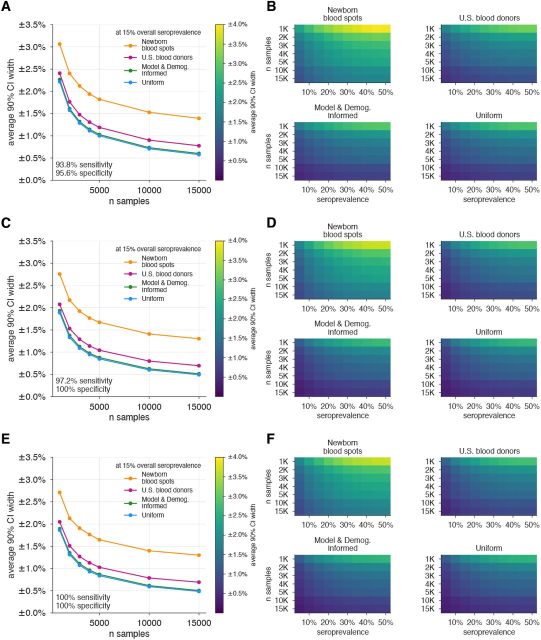
We tested the ability of the Bayesian hierarchical model described above to infer both population and subpopulation seroprevalence, even when only a convenience sample was available. The credible interval in the resulting overall seroprevalence estimates were influenced by the age demographics sampled, with the most uncertainty in the newborn dried blood spots sample set, due to the narrow age range for the mothers (Fig. 3). For such sampling strategies, which draw from only a subset of the population, our mathematical approach assumes that seroprevalence in each subpopulation does not dramatically vary and thus infers that seroprevalence in the unsampled bins is similar to that in the sampled bins but with increased uncertainty (Methods; Supplementary Text). Uncertainty was also influenced by the overall seroprevalence, such that the width of the 90% credible interval increased with higher seroprevalence for a given sample size. While test sensitivity and specificity also impacted uncertainty, central estimates of overall seropositivity were robust for sampling strategies that spanned the entire population.

Uncertainty, represented by the width of 90% credible intervals, is presented as ± seroprevalence percentage points, based on a serological test with 93% sensitivity and 97.5% specificity (Supplementary Fig. S2 depicts results for other sensitivity and specificity values). (A) Curves show the decrease in average CI widths for 15% seroprevalence, illustrating the advantages of using uniform and MDI samples over convenience samples. (B) Heatmaps show average CI widths for various total sample counts and overall seroprevalence. Convenience samples derived from newborn blood spots or U.S. blood donors improve with additional sampling but retain baseline uncertainty due to demographics not covered by the convenience sample. For the estimation of overall seroprevalence, uniform sampling is marginally superior to this example of the model and demographic informed (MDI) sampling strategy, which was designed to optimize estimation of Reff. Each point or pixel is averaged over 250 stochastic draws from the specified seroprevalence with the indicated sensitivity and specificity.
Seroprevalence estimates inform uncertainty in epidemic peak and timing
As a natural extension to use of serological data to estimate core epidemiological quantities (11–13) or to map out patterns of outbreak risk (14), the posterior distribution of seroprevalence can be used as an input to any epidemiological model, including a typical SEIR model (3), where the proportion seropositive may correspond to the recovered/immune compartment, or a more complex framework such as an age-structured SEIR model incorporating interventions like closing schools and social distancing (10,15) (Fig. 1; blue annotations). We integrated uncertainty in the posterior estimates of seroprevalence and uncertainty in model dynamics or parameters using Monte Carlo sampling to produce a posterior distribution of trajectories or key epidemiological parameter estimates (Fig. 1; black annotations).
Figure 4 illustrates how estimates of the height and timing of peak infections varied under two serological sampling scenarios and two hypothetical social distancing policies for a basic SEIR framework parameterized using seroprevalence data. Uncertainty in seroprevalence estimates propagated through SEIR model outputs in stages: larger sample sizes at a given seroprevalence resulted in a smaller credible interval for the seroprevalence estimate, which improved the precision of estimates of both the height and timing of the epidemic peak. In this case, we assumed the same serological test sensitivity and specificity as before (93% and 97.5%, respectively), but test characteristics also impacted model estimates, with more specific and sensitive tests leading to more precise estimates (Supplementary Fig. S3). Even estimations from a perfect test carried uncertainty, which corresponds to the size of the sample set (Supplementary Fig. S3).

Serological test outcomes for n = 100 tests (A; red) and n = 1000 tests (B; blue) produce (C,D) posterior seroprevalence estimates with quantified uncertainty. (E,F) Samples from the seroprevalence posterior produce a distribution of epidemic curves for scenarios of 25% and 50% social distancing (see Methods), leading to uncertainty in (G) epidemic peak and (H) timing which is mitigated in the n = 1000 sample scenario. Boxplot whiskers span 1.5 × IQR, boxes span central quartile, lines indicate medians, and outliers were suppressed.
For convenience samples from particular age groups or age-stratified serological surveys, the Bayesian hierarchical model extrapolates seroprevalence in sampled subpopulations to the overall population, with uncertainty propagated from these estimates to model-inferred epidemiological parameters of interest, such as Reff. Estimates from 1000 neonatal heel sticks or blood donations achieved more uncertain, but still reasonable, estimates of overall seroprevalence and Reff as compared to uniform or demographically informed sample sets (Fig. 5). Here, convenience samples produced higher confidence estimates in the tested subpopulations, but high uncertainty estimates in unsampled populations through our Bayesian modeling framework. In all scenarios, our framework propagated uncertainty appropriately from serological inputs to estimates of overall seroprevalence or Reff. Improved test sensitivity and specificity correspondingly improved estimation and reduced the number of samples that would be required to achieve the same credible interval for a given seroprevalence, and would similarly reduce the sampling needed to equivalent estimation of Reff (Supplementary Figs. S5 and S7).

(A-D) For four sampling strategies, n = 1000 tests were allocated to age groups with negative tests (grey) and positive tests (colors) as shown, for a test with 93% sensitivity and 97.5% specificity. The MDI strategy shown was designed to optimize estimation of Reff. (E-H) Age-group seroprevalence estimates θi are shown as boxplots (boxes 90% CIs, whiskers 95% CIs); dots indicate the true values from which data were sampled. Note the decrease uncertainty for boxes with higher sampling rates. (I) Age-group seroprevalences were weighted by population demographics to produce overall seroprevalence estimates, shown as probability densities with 90% credible intervals shaded and highlighted with dashed lines. (J) Age-group seroprevalences were used to estimate Reff under status quo ante contact patterns, shown as probability densities with 90% credible intervals shaded and highlighted with dashed lines. Dashed lines indicate true values from which the data were sampled. Each distribution depicts inference outcomes from a single sent of stochastically sampled data; no averaging is done. Note that although uniform sample allocation produces a more confident estimate of overall seroprevalence, MDI produces a more confident estimate of Reff since it allocates more samples to age groups most relevant to model dynamics.
If the subpopulation in the convenience sample has a systematically different seroprevalence from the general population, increasing the sample size may bias estimates (Supplementary Figs. S4 and S7). This can be avoided using data from other sources or by updating the Bayesian prior distributions with known or hypothesized relationships between seroprevalence of the sampled and unsampled populations.
Strategic sample allocation improves estimates
The flexible framework described in Fig. 1 enables the calculation of sample sizes for different serological survey designs. To calculate the number of tests required to achieve a seroprevalence estimate with a specified tolerance for uncertainty, and to allocate tests according to a specific subpopulation or in the context of a particular intervention, we treated the eventual estimate uncertainty as a framework output and then sought to minimize it by improving the allocation of samples (Fig. 1, dashed arrow).
Uniform allocation of samples across subpopulations is not always optimal; it can be improved upon by i) increasing sampling in subpopulations with higher seroprevalence, and ii) increasing sampling in subpopulations with higher relative influence on the quantity to be estimated. This approach, which we termed model and demographics informed (MDI), allocates samples to subpopulations in proportion to how much sampling them would decrease the posterior variance of estimates, i.e,  , where
  is the probability of a positive test in subpopulation i given test sensitivity (se), test specificity (sp), and subpopulation seroprevalence θi, and xi is the the relative importance of subpopulation i to the quantity to be estimated. When that quantity is overall seroprevalence, xi is the fraction of the population in subpopulation i; when that quantity is total infections or Reff, xi can be derived from the structure of the model itself (see Methods). If subpopulation prevalence estimates θi are unknown, sample allocation based solely on xi is recommended.
To demonstrate the effects of MDI sample allocation, we used it to design a strategy to optimize estimates of Reff and then tested the performance of its sample allocations against those of blood donations, neonatal heel sticks, and uniform sampling. MDI produced higher confidence posterior estimates (Fig. 5J, Supplementary Fig. S7). Importantly, because the relative importance of subpopulations in a model may vary based on the hypothetical interventions being modeled (e.g., the re-opening of workplaces would place higher importance on the serological status of working-age adults), MDI sample allocation recommendations may have to be derived for multiple hypothetical interventions and then averaged to design a study from which the largest variety of high-confidence results can be derived. To see how such recommendations would work in practice, we computed MDI recommendations to optimize three scenarios for the contact patterns and demography of the U.S. and India, deriving a balanced sampling recommendation (Fig. 6).

Bar charts depict recommended sample allocation for three objectives, reducing posterior uncertainty for (A,E) estimates of overall seroprevalence, (B,F) predictions from an age-structured model with status quo ante contact patterns, (C,G) predictions from an age-structured model with modified contacts representing, relative to pre-crisis levels: a 20% increase in home contact rates, closed schools, a 25% decrease in work contacts and a 50% decrease of other contacts (8, 9), and (D,H) averaging the other three MDI recommendations to balance competing objectives. Data for both the U.S. (blue; A-D) and India (orange; E-H) illustrate the impact of demography and contact structure on strategic sample allocation. These sample allocation strategies assume no prior knowledge of subpopulation seroprevalences {θi}.
Discussion
There is a critical need for serological surveillance of SARS-CoV-2 to estimate cumulative incidence. Here, we presented a formal framework for doing so to aid in the design and interpretation of serological studies. We considered that sampling may be done in varying ways, including broad initial efforts to approximate seroprevalence using convenience samples, as well as more complex and resource-intensive structured sampling schemes, and that these efforts may use one of any number of serological tests with distinct test characteristics. We further incorporated into this framework an approach to propagating the estimates and associated uncertainty through mathematical models of disease transmission (focusing on scenarios where seroprevalence maps to immunity) to provide decision-makers with tools to evaluate the potential impact of interventions and thus guide policy development and implementation.
Our results suggest approaches to serological surveillance that can be adapted as needed based on pre-existing knowledge of disease prevalence and trajectory, availability of convenience samples, and the extent of resources that can be put towards structured survey design and implementation.
In the absence of baseline estimates of seroprevalence, an initial survey will provide a preliminary estimate of population prevalence (Fig. 2). Our framework updates the ‘rule of 3’ approach (16) by incorporating uncertainty in test characteristics and can further address uncertainty from biased sampling schemes (see Supplementary Text). As a result, convenience samples, such as newborn heel stick dried blood spots or samples from blood donors, can be used to estimate population seroprevalence. However, it is important to note that in the absence of reliable assessment of correlations in seroprevalence across age groups, extrapolations from these convenience samples may be misleading as sample size increases (Supplementary Figs. S4 and S6). Uniform or model and demographic informed samples, while more challenging logistically to implement, give the most reliable estimates. The results of a one-time study could be used to update the priors of our Bayesian hierarchical model and improve the inferences from convenience samples. In this context, we note that our mathematical framework naturally allows the integration of samples from multiple test kits and protocols, provided that their sensitivities and specificities can be estimated, which will become useful as serological assays improve in their specifications.
The results from serological surveys will be invaluable in projecting epidemic trajectories and understanding the impact of introducing or stopping interventions. We have shown how the estimates from these serological surveys can be propagated into transmission models, incorporating model uncertainty as well. Conversely, to aid in rigorous assessment of particular interventions that meet accuracy and precision specifications, this framework can be used to determine the needed number and distribution of population samples via model and demographic informed sampling.
There are a number of limitations to this approach that reflect uncertainties in the underlying assumptions of serological responses and the changes in mobility and interactions that have arisen in response to public health mitigation efforts, such as ‘social distancing.’ Serology reflects past infection, and the delay between infection and detectable immune response means that serological tests reflect a historical cumulative incidence (the date of sampling minus the delay between infection and detectable response). The possibility of heterogeneous immune responses to infection and unknown dynamics and duration of immune response mean that interpretation of serological survey results may not accurately capture cumulative incidence. For COVID-19, we do not yet understand the serological correlates of protection from infection, and as such projecting seroprevalence into models that assume seropositivity indicates immunity to reinfection may be an overestimate; models would need to be updated to include partial protection or return to susceptibility.
Use of model and demographic-informed sampling schemes are valuable for projections that evaluate interventions, but are dependent on accurate parameterization. While in our examples we used POLYMOD and other contact matrices, these represent the status quo ante, and should be updated to the extent possible using other data, such as those obtainable from surveys (8, 9) and mobility data from online platforms and mobile phones (17–19). Moreover, the framework could be extended to geographic heterogeneity as well as longitudinal sampling, if, for example, one wanted to compare whether the estimated quantities of interest (e.g., seroprevalence, Reff) differ across locations or time (14).
Overall, the framework here can be adapted to communities of varying size and resources seeking to monitor and respond to the SARS-CoV-2 pandemic. Further, while the analyses and discussion focused on addressing urgent needs, this is a generalizable framework that with appropriate modifications can be applicable to other infectious disease epidemics.
Data Availability
All data and open-source code for this manuscript can be found in the github repository referenced in this paper.
Materials and Methods
Bayesian estimation of seroprevalence in a single population
For a test with sensitivity 1 − v and specificity 1 − u, and given n+ seropositive and n− seronegative results, the posterior distribution over seropositivity θ, using a uniform prior over θ, is proportional to the probability of the observed data under the binomial distribution, i.e.,
 from which we drew samples using an accept-reject algorithm (Supplementary Materials).
Bayesian estimation of seroprevalence across subpopulations
For a test with sensitivity 1 − v and specificity 1 − u, and given ni+ seropositive and ni− seronegative results for subpopulation i—set equal to zero for unsampled subpopulations—the posterior distribution over the vector of subpopulation seropositivities θ = {θi} is given by
 where we have included a hierarchy of priors. Specifically, the prior for each subpopulation seroprevalence was
  , which has expectation
  and variance
  . The hyperprior for the overall mean
  was uniform, allowing it to be dictated by the observed data. The hyperprior for the variance parameter was γ ∼Gamma(ν, scale = γ0/ν), which has expected value E[γ] = γ0 and
  . In all inferences of this study γ0 = 150 and ν = 1. Sampling from the joint posterior distribution was done using Markov chain Monte Carlo (see Supplementary Materials; (20)).
Single-population simulations and inference
For simulated sampling and inference (Fig. 2), n serological samples were drawn from a population with seroprevalence θ, including false positive and negative results as dictated by the test being modeled (see Supplementary Table S1). Given test outcomes, a posterior distribution was inferred using 1, 000 or more samples from the posterior distribution Eq. (1) using an accept-reject algorithm, and the 90% equal-tailed credible interval was recorded. Average posterior 90% CI widths were calculated using 250 technical replicates per pixel/point (Fig. 2).
For simulated SEIR model-based projections using serology, we considered a single set of n = 100 serological samples of which 16 were positive, corresponding to the expected results from a seroprevalence of θ = 0.15 and sensitivity/specificity values from the SensingSelf test kit (Supplementary Table S1). The posterior distribution Eq. (1) was then sampled 100 times using an accept-reject algorithm, and each sampled θ was used in the initial conditions of an SEIR simulation, described below. To isolate the effect of sample size alone, the outcomes of the n = 100 tests were scaled up tenfold to a total of n = 1000 tests and the above procedure was repeated. To compare differences between test kits, samples were generated as above, such that each kit produced the expected number of true/false positive/negative outcomes (Supplementary Table S1, Fig. 4, and Supplementary Fig. S3).
Age-structured simulations and inference
For simulated sampling and inference (Fig. 3), n = {ni} serological samples were allocated to subpopulations with heterogeneous seroprevalence values θ (Supplementary Table S2), shifted upward or downward to achieve the targeted overall seroprevalence. Simulated test outcomes included false positive and negative results as dictated by the test being modeled (see Supplementary Table S1). Test allocations {ni} were done in proportion to age demographics of blood donations, delivering mothers, uniformly across subpopulations, or according to a variance reduction strategy, MDI; see below. Given per-subpopulation test outcomes, 1, 000 or more samples were drawn from the posterior distribution Eq. (2) using MCMC (Supplementary Materials). Posterior distributions of overall seroprevalence were produced by a demographically weighted average of age-specific seroprevalence samples. Posterior distributions of Reff were produced by using samples of age-specific seroprevalences in the age-structured model, described below. For both overall seroprevalence and Reff, 90% equal-tailed credible intervals were recorded. Average posterior 90% CI widths were calculated using 250 technical replicates per pixel/point (Fig. 3, Supplementary Figs. S2, S4, S5, S6, S7). A single technical replicate was used to produce Fig. 5.
SEIR model with social distancing
A simple SEIR model with social distancing was used with transmission rate β = 1.75, exposure-to-infected rate α = 0.2, and recovery rate γ = 0.5, with no births or deaths, in a finite population of size N = 10, 000. Social distancing was implemented as a coefficient ρ = {0.5, 0.75}, corresponding to 50% and 25% social distancing, multiplying the contact rate between infected and susceptible populations. Integration was performed for 150 days with a timestep of 0.1 days. Initial conditions for (S, E, I, R) were (N − 20 − θN, 10, 10, θN), to simulate a fraction θ of recovered individuals, assumed to be immune. For each sampled value of θ, peak infection height and timing were extracted from forward-integrated timeseries. The model is described fully in Supplementary Materials.
Age-structured model
A model with 16-age-bins (0−4, 5−9, … 75−79) was parameterized using country-specific age-contact patterns (8, 9) and COVID-19 parameter estimates (10). The model, due to S13, included age-specific clinical fractions and varying durations of preclinical, clinical, and subclinical infectiousness, as well as a decreased infectiousness for subclinical cases. Reff for age-specific seropositivity estimates θ was calculated as the principal eigenvalue of the serology-adjusted next-generation-matrix, N (θ) = D1−θDuCDay+b, where Dx represents a diagonal matrix with entries Dii = xi, and the constants are defined a = µP + µC − fµS and b = µS. Definitions and values for model parameters are reported in Supplementary Table S2.
Model and demographics informed (MDI) sampling
MDI sampling attempts to decrease posterior uncertainty by intelligently allocating finite samples to subpopulations and is fully described in Supplementary Materials. In summary, to allocate samples to minimize posterior uncertainty of overall seroprevalence, MDI recommends  where di is the fraction of the total population in subpopulation i, with ni ∝ di in the absence of prior information about θi. To allocate samples to minimize posterior uncertainty associated with compartmental models with subpopulations, inclusive of any modeled interventions, MDI rec ommends
  where xi is the ith entry of the principal eigenvector of the model’s next generation matrix, including modeled interventions, with ni ∝ xi in the absence of prior information about θi.
Demographic and contact data
Demographic data for the U.S. and India were downloaded from the 2019 United Nations World Populations Prospects report (21). Age distribution of U.S. blood donors was drawn from a study of Atlanta donors (22). Age distribution of U.S. mothers were drawn from the 2016 CDC Vital Statistics Report, using Massachusetts as a reference state (23). Daily age-structured contact data were drawn from Prem. et al (9). All data were represented using 5-year age bins, i.e. (0 − 4, 5 − 9,…,74 − 79). For datasets with bins wider than 5 years, counts were distributed evenly into the five-year bins.
Serological test sensitivity and specificity values
Serological test characteristics were col lected from the websites of manufacturers and summarized in Supplementary Table S1. No attempt was made to test or validate manufacturer claims.
Software
All calculations were done in Python 3.7.4 and R 3.6.2. Reproduction code is open source and provided by the authors (20).
Supplementary Materials For
S1 Bayesian inference methods
S1.1 Inference of seroprevalance in a sample using an imperfect test
If a serological test had perfect sensitivity and specificity, the probability of observing n+ seropositive and n− seronegative results from n tests, given a true population seroprevalence θ, is given by the binomial distribution:

However, imperfect specificity and sensitivity require that we modify this formula. For convenience, in the remainder of this supplemental text, we will use:
Using this notation, the probability that a single test returns a positive result, given u, v, and the true seroprevalence θ, is

Substituting this per-sample probability into Eq. (S1) yields

Finally, using Bayes’ Rule, we can write the posterior distribution over seropositivity θ, given the data, the test’s parameters (24), and an uninformative (uniform) prior on θ, yielding
 where B is an incomplete beta function without normalization. In practice, to sample from this distribution, one can use an accept-reject algorithm and consider only the numerator of Eq. (S4).
S1.2 Sampling from the Bayesian hierarchical model for subpopulation seroprevalences using MCMC
We sample from the joint posterior distribution inside the integral in Eq. (2) using a Markov chain Monte Carlo (MCMC) algorithm, with univariate Metropolis-Hastings updates. We initialize the age-specific seroprevelance parameters at θi = (n+ + 1)/(ni + 2), set  equal to the sample mean of the {θi} and set γ = γ0. For each simulation, the MCMC algorithm was run for a total of 50, 100 iterations. The first 100 iterations were discarded and every 50th sample was saved to obtain 1, 000 samples from the joint posterior distribution.
S2 Model and demographic informed (MDI) sampling
The calculations that follow rely on facts from optimization theory. We briefly review these here before applying these results in what follows.
Let n = (n1, …, nK). Suppose we want to minimize a function of the form
 subject to the constraint that ∑i ni = n. Using the method of Lagrange multipliers, it can be shown that f (n) is minimized when
  . We apply this result below with various expressions for ci to determine the optimal allocation of n tests across subpopulations in order to minimize the uncertainty of quantities of interest.
S2.1 Minimizing posterior uncertainty for seroprevalence
Given age-specific seroprevalence estimates θ, the estimate for overall seroprevalence is defined as θpop = ∑i diθi, where di is the proportion of the population in group i. The uncertainty of this estimator depends on the uncertainties of the age-specific seroprevalences, which inherently depend on the number of tests ni allotted to each subpopulation. Although the posterior uncertainties of the subpopulation seroprevalences are not available in closed form, we can nevertheless approximate them using the uncertainties in the corresponding maximum likelihood estimators. Here we consider the maximum likelihood estimators based on a separate binomial model for each subpopulation, i.e models of the form Eq. (S3) where θ is replaced by θi. Note that this model assumes independence among the subpopulation seroprevalences.
The maximum likelihood estimate of θi, given ni,+ positive tests out of ni tests administered, is
 but this is only valid when both the numerator and denominator are positive, corresponding to a value of
  in the interval (0, 1). If the above estimator is computed and found to be negative, which happens when the fraction of tests that are positive is below the false positive rate, then the maximum likelihood lies at the endpoint,
  . Similarly, if the estimator is found to be greater than one,
  . These estimators are undefined if no tests are allocated to group i, i.e. when ni = 0.
Using the maximum likelihood estimators as proxies for the subpopulation posterior distributions, we can approximate the posterior variance of θpop as
 where θi is the true seroprevalence of group i. This variance equation has the form of Eq. (S5) and thus the optimal allocation of samples is given by

In the absence of knowledge about the true subpopulation seroprevalences θ, we recommend simply allocating samples with respect to the demographic information: ni ∝ di.
S2.2 Minimizing posterior uncertainty for modeling
When the primary quantity of interest is the output from a model, improved test allocation strategies can be developed by leveraging the model structure. For example, suppose the goal is accurate estimation of the total number of infected individuals at some future time point t. To avoid confusion with the identity matrix I or the subpopulation index i, let Let  denote the vector containing the number of infected individuals within each subpopulation and let the total number of infected individuals be
  . Using the next generation matrix defined in Eq. (S11) and modification as in Eq. (S12), the next generation matrix updates the vector of infected individuals per subpopulation as
 where x represents the eigenvector of N corresponding to the largest eigenvalue λ, and k is a constant k = xT h. 1 There are two helpful interpretations of this equation. First, the vector x is the principal “direction” of the next generation matrix, and repeated iterations of the dynamics in a large population will result in infected fractions that are proportional to x. In the above, we approximate the effect of N on h as kλx, an approximation which is better when λ is well separated from the second eigenvalue λ2.
A second interpretation of this result appeals to the notion of the next generation matrix N as a network in which the nodes are infected subpopulations and the directed links Nij explain the effects of an infection at node j on future infections at node i. In this network dynamical system, by calculating x we have computed the eigenvector centralities of the network’s nodes (25), which are a measure of the importance of each subpopulation in the network.
With these preliminary calculations in mind, we turn to the estimation of Ht. Because  , and because the values
  are all functions of a random variable θ, Ht is also a random variable. Our goal is to minimize its variance by strategically allocating finite samples in order to minimize the important posterior variances among the elements of θ. In plain language, some of the subpopulations are more important in shaping future disease dynamics than others, so MDI will preferentially allocate more samples to those subpopulations in a principled manner, which we now derive.
As in Eq. (S6), we approximate the posterior variance of θ by the posterior variance of the corresponding maximum likelihood estimator  . This results in the following approximation of the variance of the total number infected:
 where xi is the ith element of the principal eigenvector x. The first expression is obtained by using the approximation in Eq. (S8). The resulting variance expression has the form of Eq. (S5) and thus, ignoring constants, the optimal allocation of samples is given by

In the absence of knowledge about the true subpopulation seroprevalences θ, we recommend simply allocating samples with respect to the entries of the principal eigenvector: ni ∝ xi.
S3 Including protective seropositivity into models
S3.1 Canonical SEIR with social distancing
Let S, E, I, and R be the number of susceptible, exposed, infected, and recovered people in a population of size N, S + E + I + R = N. We model dynamics by
 where β, α, and γ represent the rates of infection, symptom onset, and recovery, respectively, as in a typical SEIR model. To model social distancing we include the contact parameter ρ ∈ [0, 1] which modulates the fraction of social contacts between S and I populations that remain. Thus, ρ = 1 represents no social distancing while while ρ = 0.5 would represent a 50% reduction in contacts. In the simulations of this paper, only ρ = 0.5, 0.75 were considered as examples of dynamics.
To parameterize this model using seroprevalence, we made the modeling assumption that seropositive individuals are immune. Noting that this is only an assumption which at present requires indepth research, we therefore placed seropositive individuals into the recovered group. In other words, for a seropositive fraction θ, with 10 individuals in the E and I compartments each, initial conditions would be,

Parameter values used in this study can be found in Supplementary Table S2.
S3.2 Age-structured (POLYMOD)
The model introduced and estimated by Davies et al (10) considers an SEIR model with sixteen 5-year age groups (0 − 4, 5 − 9, …, 75 − 80), age contacts parameterized by POLYMOD-type estimates (8, 9). In its dynamics, it includes both clinical and subclinical infections, with corresponding preclinical, clinical, and subclinical infectiousness parameters durations, and lower infectiousness among subclinical infections. To compute R0, Davies et al define the next generation matrix N as having entries
 where ui is the susceptibility of age group i; Cij is the number of age-j individuals contacted by an age-i individual per day; yi is the probability that an infection is clinical for an age-I individual; µP, µC, and µS are mean durations of preclinical, clinical, and subclinical infectiousness, respectively; and f is the relative infectiousness of subclinical cases (10). Values for all parameters are reported in Supplementary Table S2.
Protective seropositivity can be included in the model by multiplying Nij as defined above by 1 − θi, where θi is the seropositivity rate of age-group i. With this included term, we can modify Eq. (S11) as
 where Dx represents a diagonal matrix with entries Dii = xi, and the constants are defined a = µP + µC − fµS and b = µS. The effective reproductive number is then the spectral radius ρ (i.e. the largest eigenvalue λ) of the next generation matrix:

As written, Eq. (S13) represents a model component shown in Fig. 1 (blue annotations) as it maps parameters θ to a point estimate of Reff. As with the canonical SEIR model, uncertainty in the model parameters themselves can also be incorporated into overall uncertainty in Reff via Monte Carlo.
S4 Impact of sensitivity and specificity on the “Rule of 3”
Suppose we have a perfect test (u = v = 0) and when we perform n tests, zero are positive. The maximum likelihood estimate of the seroprevalence would be 0. (16) proposed a simple upper 95% confidence bound on true seroprevalence equal to 3/n.
The derivation of this rule is motivated by the following question: “What is the maximum seroprevalence under which the probability of observing zero positives in n tests is less than or equal to 5%?”. Briefly, the probability of a negative test is θ and thus the probability of observing n negative tests is (1 − θ)n. Setting this equal to 0.05 and solving for θ, we find θ = 1 − .051/n ≈ 3/n, where the approximation is based on the power series representation of the exponential function.
Now, let’s consider what happens if sensitivity and specificity are not equal to one and again zero positive tests are observed. The probability of a negative test is then 1 − u − θ(1 − u − v). An upper 95% confidence bound on the true seroprevalence is then
 where the approximation is derived in a similar manner. Notice if u > 3/n, this upper bound is less than zero. This occurs when there is inconsistency between the specified false positive rate u and the observed data; namely, this occurs when n is large enough that we would have expected at least one false positive.
Even if seroprevalence is zero, we expect to observe some number positive tests simply due to imperfect test specificity. Suppose we observe n+ positive tests from a sample of n. An approximate upper 95% confidence bound on the true seroprevalence:
Supplementary Figures

Uncertainty, represented by the width of 90% credible intervals, is presented as ± seroprevalence percentage points in heatmaps and for selected seroprevalence values, based on a serological tests with (A,D) 93.8% sensitivity and 95.6% specificity, matching the claims of a Cellex test, (B,E) 97.2% sensitivity and 100% specificity, matching the claims of an Aytu IgG test, (C,F) 100% sensitivity and specificity, representing an ideal test. complementing the results for a test with 93% sensitivity and 97.5% specificity shown in the main text (Fig. 2). See Supplementary Table S1 for details on serological test kits.

Uncertainty, represented by the width of 90% credible intervals, is presented as ± seroprevalence percentage points, based on a serological tests with (A,B) 93.8% sensitivity and 95.6% specificity, matching the claims of a Cellex test, (C,D) 97.2% sensitivity and 100% specificity, matching the claims of an Aytu IgG test, (E,F) 100% sensitivity and specificity, representing an ideal test. complementing the results for a test with 93% sensitivity and 97.5% specificity shown in the main text (Fig. 3). (A,C,E) Curves show the decrease in average CI widths for 15% seroprevalence, illustrating the advantages of using uniform and MDI samples over convenience samples. (B,D,F) Heatmaps show average CI widths for various total sample counts and overall seroprevalence. Convenience samples derived from newborn blood spots or U.S. blood donors improve with additional sampling but retain baseline uncertainty due to demographics not covered by the convenience sample. For the estimation of overall seroprevalence, uniform sampling is marginally superior to this example of the model and demographic informed (MDI) sampling strategy, which was designed to optimize estimation of Reff. Each point or pixel is averaged over 250 stochastic draws from the specified seroprevalence with the indicated sensitivity and specificity.

Serological test outcomes for (A) n = 100 tests and (B) n = 1000 tests produce are shown as bar graphs for four tests with sensitivity and specificity values as indicated. Serological test samples were not generated stochastically but instead according to expectation to highlight how sensitivity and specificity affect inference. Posterior seroprevalence estimates for (C) n = 100 and (D) n = 1000 scenarios reveal that Bayesian estimate place posteriors over the correct values (15%) but with uncertainty that depends on n (compare C to D) and on test characteristics (compare peak heights of yellow and purple to blue and orange). Samples from the seroprevalence posterior produce a distribution of epidemic curves for scenarios of 25% and 50% social distancing (see Methods), leading to uncertainty in (E) height of epidemic peak and (F) timing of epidemic peak. Uncertainty is mitigated but not eliminated in the n = 1000 scenario, just as uncertainty is mitigated but not eliminated using a perfect serological test. Boxplots reflect 100 samples from SEIR dynamimcs; whiskers span 1.5×IQR, boxes span central quartile, lines indicate medians, and outliers not shown. See Methods for SEIR simulation details and parameters.

Credible interval coverage, defined as the fraction of posterior credible intervals that covered the true parameter used to generate the data, are shown for four sampling strategies (columns, colors) and four test kits (rows), with sensitivity and specificity values as indicated; see legends. Each point represents the fraction of credible intervals which covered the planted value for the indicated overall seroprevalence value (see annotations on plots) at the specified number of serological samples n, out of a total of 250 independent trials. The estimated coverage from a perfectly calibrated posterior will have coverage fractions within 0.9±0.37 (grey bands) 95% of the time. Some seroprevalence values are plotted in black simply to guide the eye. The MDI strategy shown was designed to optimize estimation of Reff.

Credible intervals were calculated for data generated according to four sampling strategies (columns, colors) and four test kits (rows), with sensitivity and specificity values as indicated; see legends. Each point represents the average width of the intervals for the indicated overall seroprevalence value (see annotations on plots) at the specified number of serological samples n, out of a total of 250 independent trials. Some seroprevalence values are plotted in black simply to guide the eye. The MDI strategy shown was designed to optimize estimation of Reff. Sampling strategies that resulted in posterior credible intervals with inaccurate coverage (see Supplementary Fig. S4) are crossed out.

Credible interval coverage, defined as the fraction of posterior credible intervals that covered the true parameter used to generate the data, are shown for four sampling strategies (columns, colors) and four test kits (rows), with sensitivity and specificity values as indicated; see legends. Each point represents the fraction of credible intervals which covered the planted value for the indicated overall seroprevalence value (see annotations on plots) at the specified number of serological samples n, out of a total of 250 independent trials. The estimated coverage from a perfectly calibrated posterior will have coverage fractions within 0.9±0.37 (grey bands) 95% of the time. Some seroprevalence values are plotted in black simply to guide the eye. The MDI strategy shown was designed to optimize estimation of Reff.

Credible intervals were calculated for data generated according to four sampling strategies (columns, colors) and four test kits (rows), with sensitivity and specificity values as indicated; see legends. Each point represents the average width of the intervals for the indicated overall seroprevalence value (see annotations on plots) at the specified number of serological samples n, out of a total of 250 independent trials. Some seroprevalence values are plotted in black simply to guide the eye. The MDI strategy shown was designed to optimize estimation of Reff. Sampling strategies that resulted in posterior credible intervals with inaccurate coverage (see Supplementary Fig. S6) are crossed out.
Supplementary Tables
Sensitivity and specificity values were taken from manufacturer’s claims as of April 9, 2020, compiled by the Johns Hopkins Center for Health Security1.
This table is divided into two sections. The top section corresponds to the parameters of the single-population SEIR model. The bottom section corresponds to the parameters used in the age-structured SEIR model. Contact matrices Cij used in this manuscript were, in particular, those corresponding to the United States of America and India. Values for yi, the probability that an infection is clinical for an age-i individual, were generated by using three control points for young, middle and old age, then interpolating between them with a cosine-smoothing function, as described in (10). Equations for models can be found in Supplementary Text. Test kit sensitivity and specificity values are provided in Supplementary Table S1.
Acknowledgments
The authors wish to thanks Nicholas Davies, Laurent Hébert-Dufresne, Johan Ugander, Arjun Seshadri, and the BioFrontiers Institute IT HPC group. The work was supported in part by the Morris-Singer Fund for the Center for Communicable Disease Dynamics at the Harvard T.H. Chan School of Public Health.
Footnotes
↵1 The next generation matrix N is non-negative and satisfies the conditions of the Perron-Frobenius theorem which means that it has a largest eigenvalue λ—for a next generation matrix, R0 = λ—which is greater than or equal to all other eigenvalues, with a corresponding eigenvector x of non-negative components. This means that repeated applications of N to any initial vector that is not orthogonal to x will become increasingly parallel to x at a rate of λ/|λ2| per iteration, where λ2 is the second largest eigenvalue of N. This is the basis of the so-called Power Method which repeatedly applies the matrix to find the largest eigenvalue and its corresponding eigenvector.


