Estimation of airborne viral emission: quanta emission rate of SARS-CoV-2 for infection risk assessment

2.1. Estimation of the quanta emission rate

The approach proposed in the present work is based on the hypothesis that the droplets emitted by the infected subject have the same viral load as the sputum. Therefore, if the concentration of the virus in the sputum and the quantity of droplets emitted with dimensions less than 10 µm is known, the viral load emitted can be determined through a mass balance. In particular, the viral load emitted, expressed in terms of quanta emission rate (ER_q, quanta h⁻¹), was evaluated as: where c_v is the viral load in the sputum (RNA copies mL⁻¹), V_br is the volume of exhaled air per breath (cm³; also known as tidal volume), N_br is the breathing rate (breath h⁻¹), N_d is the droplet number concentration (part. cm⁻³), and V_d(D) is the volume of a single droplet (mL) as a function of the droplet diameter (D). Information about the viral load in terms of quanta is essential as the quantum represents the “viral load” considered in engineering science: in other words, an infected individual constantly generates a number of infectious quanta over time, where a “quantum” is defined as the dose of airborne droplet nuclei required to cause infection in 63% of susceptible persons.

The volume of the droplet (V_d) was determined on the basis of data obtained experimentally by (Morawska et al., 2009): they measured the size distribution of droplets for different expiratory activities (e.g. breathing, whispering, counting, speaking), recognizing that such droplets present one or more modes occurring at different concentrations. In particular, in the study a particle size distribution with four channels was considered with midpoint diameters of D₁=0.8, D₂=1.8, D₃=3.5, and D₄=5.5 µm. As an example, speaking was recognized as producing additional particles in modes near 3.5 and 5.5 µm. These two modes became even more pronounced during sustained vocalization. Details of the aerosol concentrations at the four channels of the size distribution during each expiratory activity are reported in Table 1. The midpoint diameters of each channel were used to calculate the corresponding volume of the droplets.

Based on the results obtained by (Morawska et al., 2009), equation (1) can be simplified as: where j indicates the different expiratory activities considered (namely whispered counting, voiced counting, speaking, breathing) and IR (m³ h⁻¹) is the inhalation rate, i.e. the product of breathing rate (N_br) and tidal volume (V_br), which is a function of the activity level of the infected subject. The quanta emission rate from equation (2) can vary in a wide range depending on the virus concentration in the mouth, the activity level, and the different types of expiration. Regarding the inhalation rate effect, the quanta emission rate calculations are shown for three different activity levels (resting, standing, and light exercise) in which the inhalation rates, averaged between males and females, are equal to 0.36, 0.54, and 1.16 m³ h⁻¹, respectively (Adams, 1993; International Commission on Radiological Protection, 1994).

2.2. A demonstration application: the containment measures for the spread of SARS-CoV-2 in Italy

The pandemic of a novel human coronavirus, now named Severe Acute Respiratory Syndrome CoronaVirus 2 (SARS-CoV-2 throughout this manuscript), emerged in Wuhan (China) in late 2019 and then spread rapidly in the world (https://www.who.int/emergencies/diseases/novel-coronavirus-2019). In Italy, an outbreak of SARS-CoV-2 infections was detected starting from 16 cases confirmed in Lombardy (a northern region of Italy) on 21 February. The Italian government has issued government a decree dated 11 March 2020 concerning urgent measures to contain the contagion throughout the country. This decree regulated the lockdown of the country to counteract and contain the spread of the SARS-CoV-2 virus by suspending retail commercial activities, with the exception of the sale of food and basic necessities. It represents the starting point of a system with imposed constraints. Among the measures adopted for the containment of the virus in Italy, great importance was placed on the safe distance of 1 m (also known as “droplet distance”). This distance was actually indicated by the World Health Organization as sufficient to avoid transmission by air, without any reference to the possibility of transmission over greater distances indoors (https://www.who.int/emergencies/diseases/novel-coronavirus-2019). With this measure, along with the opening of only primary commercial establishments (such as pharmacies, supermarkets, banks, post offices) and the closure of restaurants, the Italian government has adopted the concept of spacing (known as “social distancing”) to prevent the spread of the infection. Obviously, this limit per se would have no influence on the reduction of airborne transmission of the infection in indoor environments since this distance is compatible with the normal gathering of people in commercial establishments. Actually, on an absolutely voluntary basis, and despite the continuous denials by the government on the risk of indoor airborne transmission, commercial associations have changed the methods of accessing their commercial spaces such as restaurants, pharmacies, supermarkets, post offices, and banks; for example, by forcing customers to queue outside. It is clear that the best choice in containing an epidemic is a total quarantine which, however, appears to have enormous costs and social impacts, especially in Western countries.

To show the possible effect of the measures imposed by the Italian government (i.e. lockdown), the infection risk in different indoor microenvironments for the exposed population due to the presence of one contagious individual was simulated, adopting the infection risk model described in section 2.2.1. In particular, the risk expressed in terms of basic reproduction number (R₀) was derived from the quanta concentration and the infection risk; indeed, R₀ represents the average number of secondary infections produced by a typical case of an infection in a population where everyone is susceptible (Rothman et al., 2008).

The indoor microenvironments considered here were a pharmacy, supermarket, restaurant, post office, and bank whose dimensions are summarized in Table 2. Two different exposure scenarios were simulated for each microenvironment: before lockdown (B) and after lockdown (A). In the simulation of the scenario before lockdown, the microenvironments were run with no particular recommendations; thus, people enter the microenvironments and queue indoors, often resulting in overcrowded environments. Since most of the indoor microenvironments in Italy are not equipped with mechanical ventilation systems, the simulations were performed considering two different situations: natural ventilation (a typical value for an Italian building equal to 0.2 h⁻¹ was adopted, with reference to (d’Ambrosio Alfano et al., 2012; Stabile et al., 2017)) and mechanical ventilation (calculated according the national standard, UNI 10339 (UNI, 1995), as a function of the crowding index and the type of indoor microenvironment). The scenario after lockdown was tested considering the typical solutions adopted (on a voluntary basis) by the owners of stores and offices – reduced personnel, a reduced number of customers inside the microenvironment, customers forced to queue outdoors, and doors kept open. The scenario after lockdown was also tested for both natural ventilation and mechanical ventilation; in this case a slight increase in the air exchange rate (AER) for natural ventilation (0.5 h⁻¹) was considered in order to take into account that the door was always kept open. The restaurant was not tested in the scenario after lockdown since such commercial activity was closed down as a consequence of the lockdown. For all the scenarios considered in the simulations, the infected individual was considered to enter the microenvironment as the first customer (alone or along with other individuals according to the scenarios summarized in Table 2). All the scenarios were simulated taking into account that the virus is able to remain viable in the air for up to 3 hours post aerosolization as recently detected by (van Doremalen et al., 2020); thus, if the infected individual remained inside the environment for 10 minutes (e.g. pharmacy), the calculation of the quanta concentration, infection risk, and R₀ was performed for up to 3 hours and 10 minutes (named “total exposure time” in Table 2). For restaurants the calculation was performed for 3 hours considering that after 3 hours (i.e. two groups remaining inside for 1 hour and 30 minutes one after the other) the microenvironment was left empty.

3.1. The quanta emission rate

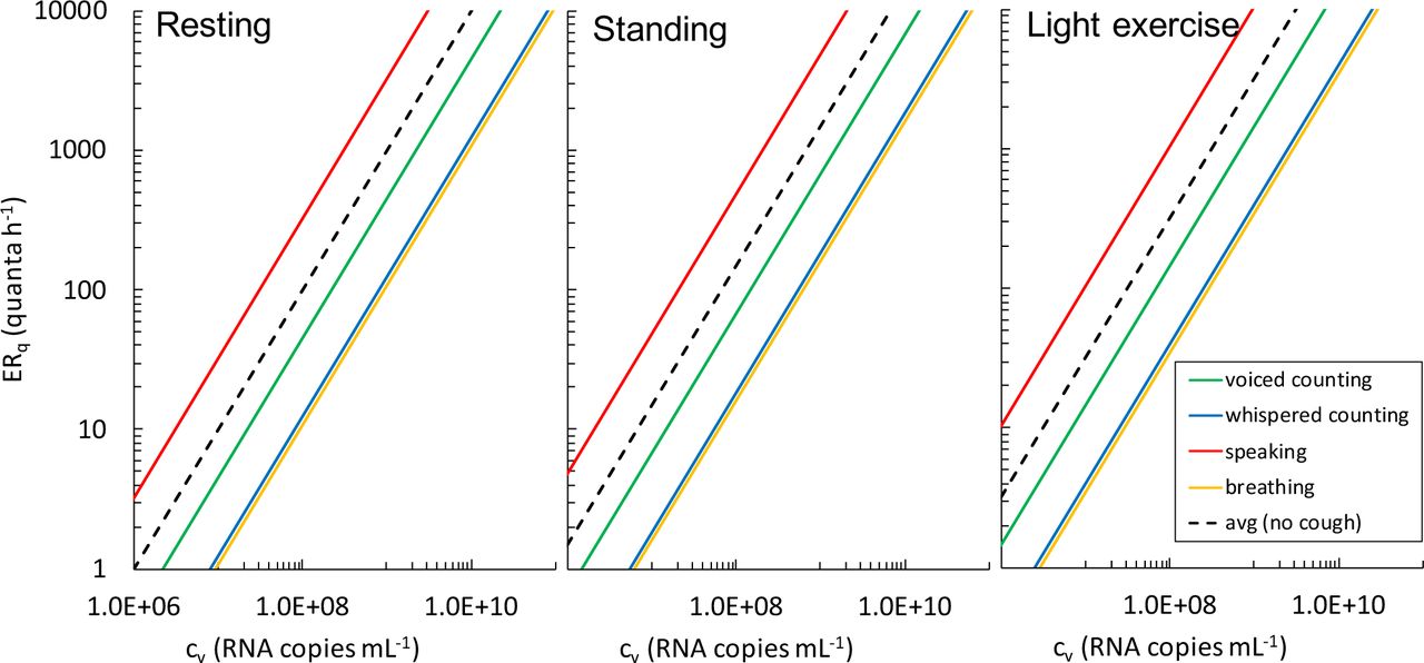
As discussed in the Materials and methods section, the quanta emission rate, ER_q, depends on several parameters. In Figure 1 the ER_q (quanta h⁻¹) trends are reported as a function of the viral load in the sputum (c_v, RNA copies mL⁻¹) for different expiratory activities (whispered counting, voiced counting, speaking, breathing) and different activity levels (resting, standing, light exercise). To represent the large variabilities (over several orders of magnitude) of ER_q as a function of c_v, the graph is reported on a bi-logarithmic scale.

• Download figure
• Open in new tab

Figure 1.

ERq (quanta h⁻¹) trends as a function of the viral load in sputum (cv, RNA copies mL⁻¹) for different respiratory activities (whispered counting, voiced counting, speaking, breathing) and different activity levels (resting, standing, light exercise). The average (avg) value of the respiratory activities considered was also reported.

To benchmark the proposed approach for the estimation of the quanta emission rate, we considered the case of seasonal influenza for which more data are available in terms of both viral load in sputum and quanta emission rate. As an example, (Hirose et al., 2016) found an average value of RNA concentration in sputum for influenza equal to 2.38×10⁷ copies mL⁻¹. Thus, applying the findings of the proposed approach in the case of a standing subject, a corresponding ER_q varying between 3.7 (breathing) and 114 quanta h⁻¹ (speaking) is estimated: this value is in good agreement with the quanta emission rates for influenza found in the scientific literature, from 2 to 128 quanta h⁻¹ with a most frequent value of 67 quanta h⁻¹ (Knibbs et al., 2012). Such variability in the quanta emission rates for influenza is due both to the method used to calculate it (Rudnick and Milton, 2003) and, especially, the viral load of the subject and the type of respiratory activity, which is typically not reported and discussed.

With reference to SARS-CoV-2 infection, researchers have recently found values for the viral load in the mouth between 10² and 10¹¹ copies mL⁻¹, also variable in the same patient during the course of the disease (Pan et al., 2020; To et al., 2020; Woelfel et al., 2020). (Rothe et al., 2020) reported a case of SARS-CoV-2 infection acquired outside Asia in which transmission appears to have occurred during the incubation period in the index patient. A high viral load of 10⁸ copies mL⁻¹ was found, confirming that asymptomatic persons are potential sources of SARS-CoV-2 infection; this may warrant a reassessment of the transmission dynamics of the current outbreak. Table 3 lists the quanta emission rates (ER_q) for a SARS-CoV-2 infected asymptomatic subject as a function of activity level (resting, standing, and light exercise) and respiratory activity (voiced counting, whispered counting, speaking, breathing). The data confirm the huge variations in the quanta emission rate, with the lowest value being for breathing during resting activity (10.5 quanta h⁻¹) and the highest value being for speaking during light activity (more than 1000 quanta h⁻¹).

3.2. Results of the demonstration application

In this section, the results of the simulations performed for the microenvironments and exposure scenarios described in section 2.2 and summarized in Table 2 are reported.

3.2.1. Infection risk and R₀ for different indoor environments and exposure scenarios

As an illustrative example, Figure 2 shows the quanta concentration (n(t)) and infection risk (R) trends as a function of time for two different exposure scenarios simulated for the pharmacy, i.e. before lockdown (B) in natural (NV) and mechanical ventilation (MV) conditions. The trends clearly highlight that the presence of the infected individual remaining inside for 10 minutes leads to an increase in the quanta concentration in the volume: in particular, a higher peak of quanta concentration was recognized, as expected, for reduced ventilation (NV) with respect to the mechanical ventilation (MV). People entering the pharmacy after the infected individual are exposed to a certain quanta concentration during their 10-min time, and the resulting risk for their exposure (evaluated through equation (4)) is just a function of the quanta concentration trend. For example, people entering the microenvironment around the quanta concentration peak are at a higher risk than people entering the pharmacy later. Figure 2 shows an example of a customer entering at min 26 and leaving at min 36: the risk for this 10-min exposure is 2.4% in natural ventilation conditions and 1.0% in mechanical ventilation conditions. During the entire exposure time of such a scenario (3 hours and 10 minutes), 179 customers (after the infected individual) enter the pharmacy and each of them receive their own risk. In particular, the average risk of the 179 customers is 2.0% for NV conditions and 0.4% for MV conditions, then leading to a R₀ (among the customers) of 3.52 and 0.68, to which must be added the R₀ of the five pharmacists exposed for the entire period. Similar trends, not shown here graphically for the sake of brevity, were obtained for all the scenarios investigated, then leading to the evaluation of the R₀ for each of them as described in the methodology section.

• Download figure
• Open in new tab

Figure 2.

Details of application of the proposed approach in the calculation of quanta concentrations, n(t), and infection risks, R, in the pharmacy environment for the exposure scenarios before lockdown (B) in natural (NV) and mechanical ventilation (MV) conditions. The graph shows the entry of the infected individual (first 10 minutes) and the risk for a customer entering the microenvironment at min 26 and remaining inside for 10 minutes. The trends are shown for up to 100 minutes to highlight the peaks of the n(t) and R values.

Figure 3 shows the reproduction number (R₀) data calculated for all the exposure scenarios and microenvironments under investigation (summarized in Table 2). The R₀ data were calculated for an asymptomatic SARS-CoV-2 infected subject (c_v=1×10⁸ copies mL⁻¹) while standing; in particular, the average ER_q value among the different respiratory activities was considered (147 quanta h⁻¹, Table 3). The exposed subjects were also considered to be standing (IR=0.54 m³ h⁻¹). The graph clearly highlights some critical exposure scenarios and microenvironments. Indeed, in all the microenvironments, a R₀>1 was estimated for all the exposure scenarios before lockdown (B) when the ventilation relied only upon the building being airtight (i.e. natural ventilation conditions): R₀ was equal to 5.55, 3.51, 59.3, 5.59, and 6.04 for pharmacy, supermarket, restaurant, post office, and bank, respectively. The huge value for the restaurant is obviously due to the simultaneous co-presence of many people (80 customers and 4 waiters) and to the long exposure time (1 h and 30 min in the current simulations). This situation is obviously improved if mechanical ventilation systems are adopted, but the R₀ is still higher than 1 (R₀=3.40). Similar results are obviously expected for all the indoor environments characterized by high crowding indexes and long-lasting exposures such as schools, swimming pools, gyms – venues that, in fact, were also concomitantly locked down by the government. Actually, adopting mechanical ventilation solutions that purportedly provide an adequate indoor air quality (i.e. providing AER values suggested by the standards (UNI, 1995)) did not satisfactorily reduce the R₀ in the other microenvironments investigated. Indeed, the R₀ values obtained from the simulations performed for the pharmacy, supermarket, post office, and bank equipped with mechanical ventilation systems in the conditions before lockdown, with mechanical ventilation in operation, were still >1.

• Download figure
• Open in new tab

Figure 3.

R₀ calculated for all the exposure scenarios (natural ventilation, mechanical ventilation; before lockdown, after lockdown) and microenvironments (pharmacy, supermarket, restaurant, post office, bank) under investigation considering an asymptomatic SARS-CoV-2 infected subject (cv=1×10⁸ copies mL⁻¹) while standing (IR=0.54 m³ h⁻¹; ERq=147 quanta h⁻¹) and the exposed population, also standing.

The new regulations and methods of accessing the indoor environments that were applied in the conditions after lockdown (i.e. queuing outside, limited time spent in the environments, lower crowding index) were very effective; indeed, the R₀ values were reduced by roughly 80%–90% (for both natural and mechanical ventilation conditions) with respect to the corresponding pre-lockdown scenarios.

As an example, for the natural ventilation scenario, the only critical microenvironment was the bank, since the R₀ was >1; this was due to a crowding index that was higher than the post-office, which had a larger floor area but same number of customers. In contrast, all the R₀ values for indoor environments equipped with mechanical ventilation systems were much lower than 1 (0.18, 0.12, 0.15, and 0.30 for pharmacy, supermarket, post office, and bank, respectively). Therefore, if in a single day the infected individual visited different environments, the resulting R₀ would be lower than 1 only if all the microenvironments were equipped with mechanical ventilation systems. Once again, these results highlight the importance of proper ventilation of indoor environments and are in line with the scientific literature that recognizes the importance of ventilation strategies in reducing indoor-generated pollution (Stabile et al., 2017)(Stabile et al., 2019).

The values obtained with this approach could vary significantly as a function of (i) the activity levels of both the infected subject and the exposed subjects; and (ii) the viral load in the sputum of the infected subject; therefore, in future studies, more specific exposure scenarios could be simulated on the basis of the findings proposed and discussed in this study.