Inferring transmission trees to guide targeting of interventions against visceral leishmaniasis and post-kala-azar dermal leishmaniasis

Pairwise transmission rates

Susceptible individuals become infected either from pre-symptomatically infected individuals, from symptomatic VL cases, PKDL cases, asymptomatic individuals, or ‘background’ (unexplained) transmission. The transmission rate, or ‘infection pressure’, between an infected individual j and a susceptible individual i at time t is given by: where β is the rate constant for spatial transmission between infected and susceptible individuals; K(d_ij) is the spatial kernel function that scales the transmission rate by the distance d_ij between individuals i and j; δ (≥0) is a rate constant for additional within-household transmission; 𝟙_ij is an indicator function for individuals living in the same household, i.e. and h_j (t) is the infectiousness of j at time t. Individuals are assumed to be stationary in their households when transmission to and from sandflies occurs (since the vast majority of sandfly biting occurs at night when individuals are asleep in, or directly outside, their homes (8–13)), so that the distances between them d_ij are fixed when transmission takes place. However, the changes in the distances between individuals that occur when individuals migrate is incorporated into the model (by calculating the distances between migrators and all other individuals both when they are in their first household and when they are in their second household).

• Download figure
• Open in new tab

Fig. S1.

Individual-level spatiotemporal transmission model. (A) States in the model (S = susceptible, 𝒜 = asymptomatically infected, ε = pre-symptomatically infected, ℐ = symptomatic VL, 𝒟 = dormantly infected, 𝒫 = PKDL and ℛ = recovered). Squares represent fully observed states, rounded-edge squares partially observed states, and circles unobserved states. p_I = probability of symptomatic infection, λ_i t = total infection pressure on susceptible individual i at time t. (B) Relative infectiousness over time of individual passing through top pathway (symptomatic infection) in (A). Diagram not to scale and shown assuming that pre-symptomatic individuals are infectious and VL case developed macular PKDL. (C) The total infection pressure λ_i(t) on a susceptible individual i at time t is the sum of the individual infection pressures on them from infectious individuals around them (here j₁, j₂ and j₃), which are a function of how far away they are (depicted by the curves), the time since their infections and whether their infection is symptomatic or asymptomatic. d_i1 = distance between i and j₁.

Since we found little difference in the goodness of fit of the model (based on the Deviance Information Criterion (DIC)) between an exponentially decaying spatial kernel and a Cauchy-type kernel in our previous study (1) (the exponential kernel gave a marginally better fit), we use the exponential kernel here: where 1/α is the distance decay rate (per m) in transmission risk (so smaller values of α correspond to a faster decrease in risk with distance), and K₀ is a normalisation constant, defined such that which reduces correlation between α and β and thus improves the mixing of the MCMC chain. However, unlike in our previous study, we allow the possibility of transmission between individuals in different paras (hamlets). The reason for this is that surveying of neighbouring paras was more complete in the two clusters of paras in the present study, and thus some minimum inter-para household distances were less than intra-para household distances and within the maximum reported flight range of P. argentipes sandflies (a few hundred metres (14–17)), so transmission between neighbouring surveyed paras may have occurred.

Infectiousness over time

There is relatively little data available on the infectiousness of individuals in different L. donovani infection states over time. We therefore assume that the infectiousness of individuals remains constant within each state and individuals in the same state have the same probability of passing on infection, such that an individual’s infectiousness over time takes the form of a step function (Fig. S1B). The relative infectiousness of asymptomatic individuals compared to VL cases, h₄, is assumed to take a fixed value between 0 and 0.02 based on estimates from previous modelling studies (3, 4, 18) and preliminary results from xenodiagnosis studies that have so far not found infection in flies fed on asymptomatically infected individuals (19). We test different values of h₄ to assess whether asymptomatic individuals are in fact infectious towards sandflies (see Model Comparison below). In the absence of data on the relative infectiousness of pre-symptomatic individuals and asymptomatic individuals, we take the relative infectiousness of pre-symptomatic individuals, h₀, to be the same as that of asymptomatic individuals (i.e. h₀ = h₄).

One-hundred and thirty-eight of the 190 PKDL cases underwent one or more examinations by a trained physician to determine the type and extent of their lesions (Table S1). Data from a recent xenodiagnosis study in Bangladesh (20) on 47 PKDL patients (21 nodular and 26 macular/papular) and 15 VL patients is used to assign infectiousness to these cases according to their lesion type (macular/papular, plaque, or nodular) (Table S1). The results of the xenodiagnosis study suggest that infectiousness of PKDL increases with lesion severity and macular/papular PKDL cases are less infectious towards sandflies than VL cases but nodular PKDL cases more so. As plaques were not treated as a separate lesion type in the study, but are intermediate in severity between macular/papular lesions and nodular lesions (21), a value halfway between the infectiousness of macular/papular PKDL cases and nodular PKDL cases is assigned to these individuals. The 52 PKDL cases that were not physically examined during the study are assigned an average of the infectiousnesses of the different lesion types (weighted by frequency amongst the examined cases). Although it is not known for certain whether treated VL cases who subsequently relapse or develop PKDL are uninfectious following treatment, we assume dormantly infected individuals are uninfectious, based on rapid decreases in parasitaemia observed in VL cases following the start of treatment (22, 23)). We assume that relapse cases are as infectious upon relapse as in their first clinical episode, as relapse appears to be associated with resurgence in parasitaemia to high parasite loads (23, 24). Over half (100/190=53%) of the PKDL cases did not receive treatment, and of these 49 self-resolved in a median time of 20 months (interquartile range (IQR) 14–32 months). These cases are assumed to have remained infectious until their lesions resolved, while treated PKDL cases are assumed to have stopped being infectious once their treatment commenced (25).

Thus, individual j ‘s infectiousness at time t is given by

Incubation period

Following previous work (1), we model the incubation period as negative binomially distributed NB(r, p) with fixed shape parameter r = 3 and ‘success’ probability parameter p, and support starting at 1 (such that the minimum incubation period is 1 month): We estimate p in the MCMC algorithm for inferring the model parameters and missing data (see below).

VL onset-to-treatment time distribution

Several VL cases with onset before 2002 have missing symptom onset and/or treatment times (only their onset year is recorded), and may therefore have been infectious at the start of the study period. In order to be able to infer the onset-to-treatment times of these cases, , in the MCMC algorithm (see below) we model the onset-to-treatment time distribution as a negative binomial distribution NB(r₁, p₁) and fit to the onset-to-treatment times of all VL cases for whom both onset and treatment times were recorded (Figure S2A): to obtain r₁ = 1.34 and p₁ = 0.38 (corresponding to a mean onset-to-treatment time of 3.2 months).

Asymptomatic infection duration

Neither the infection or recovery time of asymptomatically infected individuals is observed, so we need to specify a distribution for the asymptomatic infection duration in order to infer their recovery times. Based on a previous multi-state Markov model of the natural history of VL (26), in which it was assumed that the duration of asymptomatic infection is exponentially distributed and its mean was estimated as approximately 5 months, we assume the asymptomatic infection duration, AIP_j = R_j − A_j, follows a geometric distribution (the discrete analog of the exponential distribution) Geom(p₂), with a minimum duration of 1 month and a mean of 5 months : The choice of the geometric distribution is partly motivated by the fact that it is a memoryless distribution, i.e. P(AIP_j > s + t |AIP_j > s) = ℙ(AIP_j > t). This simplifies the estimation of recovery times for initially asymptomatically infected individuals (see Model for initial status of non-symptomatic individuals below) in the MCMC algorithm as it means that the probability that an initially asymptomatically infected individual remains infected for a further t months is the same as if they were infected in month 0 regardless of when they were infected.

Dormant infection duration

Sixteen (8.4%) of the 190 PKDL cases reported no prior history of VL, and are assumed to have been previously asymptomatically infected. We assume that their duration of dormant infection prior to PKDL and that of VL cases who develop PKDL follow the same negative binomial distribution, NB(r₃, p₃), and estimate r₃ and p₃ by fitting to the observed VL-treatment-to-PKDL-onset times by maximum likelihood estimation (Figure S2B). Unlike for the incubation period, we take 0 months to be the minimum duration of dormant infection, since two VL cases developed PKDL in the same month as they were treated for VL, and one had simultaneous VL and PKDL. Thus the probability mass function (PMF) is: where r₃ = 1.73 and p₃ = 0.065 (corresponding to a mean duration of dormant infection of 25 months).

• Download figure
• Open in new tab

Fig. S2.

Observed and fitted negative binomial distributions of (A) VL onset-to-treatment time and (B) VL-treatment-to-PKDL-onset time.

Time to relapse and relapse duration

Forty-five VL cases suffered treatment failure or relapse during the study. Of these, 16 were treated with miltefosine and 29 with sodium stiboglucanate (SSG). Of those treated with miltefosine, 15 were treated with counterfeit drug in 2008 (27) and all but one of these cases reported no gap between the start of treatment and recurrence of symptoms (the other case reported a gap of 30 days). We assume that individuals without any gap between treatment and symptom recurrence suffered treatment failures, and that their infectiousness continued for 1 month following the start of treatment until they were treated with SSG. The gap between the start of treatment and new symptoms occurring was recorded for 7 of the cases originally treated with SSG or miltefosine from a clinical trial, and was non-zero in all cases. We assume that all cases not recorded as having immediate recurrence of symptoms suffered treatment relapse and that the time to relapse follows a geometric distribution Geom(p₄) with PMF: where fitting to the recorded gaps gives p₄ = 0.13 (corresponding to a mean time to relapse of 7.9 months). Relapse cases are assumed to be uninfectious from their treatment month to their relapse time and their duration of symptoms upon relapse is assumed to follow the same distribution as the onset-to-treatment time for a first VL episode (Eq. (5)). We assume all relapse cases were treated for relapse before the end of the study, since the latest treatment time for primary VL in a case that subsequently relapsed was April 2009.

Infection pressure

The total infection pressure on susceptible individual i at time t is given by the sum of the infection pressures on them from all infectious individuals (VL cases, PKDL cases, pre-symptomatic individuals and asymptomatic individuals) at time t in Eq. (1) (see Fig S1C) plus a constant background transmission rate ϵ to account for unexplained infections due to non-explicitly modelled factors (e.g. due to short-term movement of individuals) where Inf (t) = ε (t) ∪𝒜 (t) ∪ℐ (t) ∪𝒫 (t) is the set of all individuals infectious at time t. The transmission process is thus described by a discrete-time approximation to an inhomogeneous Poisson process with rate λ(t) =∑_i∈S(t) λ_i(t). The probability of susceptible individual i remaining susceptible in any particular month t is: while the probabilities of pre-symptomatic or asymptomatic infection in month t given susceptibility up to month t − 1 are, respectively:

Asymptomatic infection times

In order to account for the uncertainty in the parameter estimates due to the missing asymptomatic infection and recovery times, we need to estimate which individuals were asymptomatically infected during the study and when they were infected, as part of the MCMC algorithm. To do this, we assign every non-symptomatic individual j in the population an asymptomatic infection time and recovery time pair, (A_j, R_j) ∈ {V_j, V_j + 1,…, W_j − 1,T + 1} ×{A_j + 1, A_j + 2,…, W_j − 1,T + 1}, where asymptomatic infection and recovery before the study is labelled as (A_j, R_j) = (0, 0), asymptomatic infection before and recovery during/after the study is labelled as (A_j, R_j) = (0, s), (s 1,…,T + 1), and no asymptomatic infection before or during the study is labelled as (A_j, R_j) = (T + 1,T + 1). Posterior distributions for the asymptomatic infection and recovery time pairs are then estimated in the MCMC algorithm by proposing moves for these pairs and accepting/rejecting them based on the Metropolis-Hastings acceptance probability. The posterior distribution for which non-symptomatic individuals were asymptomatically infected during the study can be estimated from the proportion of time in the MCMC chain each individual spends in states other than (T + 1,T + 1). Since every non-symptomatic individual has an infection and recovery time pair, with a finite set of possible values, the dimension of the model remains fixed and reversible jump MCMC (RJMCMC) is not required. We note, however, that the algorithm described below for updating the asymptomatic infection and recovery time pairs is equivalent to a classical RJMCMC algorithm in which only individuals that are asymptomatically infected before or during the study have asymptomatic infection and recovery times and the number of asymptomatic infections varies as asymptomatic infection times are added or removed in the steps of the algorithm (31–34). As in the RJMCMC algorithm, the likelihood can be higher in the initial iterations of the chain than the value it ultimately converges to in our approach since the number of asymptomatic infections in the likelihood changes as the number of pairs corresponding to asymptomatic infection before or during the study changes, despite the fixed dimension of the parameter space.

In order to sample effectively from the posterior distribution of the asymptomatic infection and recovery times, we need to use a proposal distribution that allows us to efficiently navigate the very large space of possible asymptomatic infection and recovery time pairs. We therefore use the running estimate of the total infection pressure on each individual, averaged over the history of the MCMC chain, to propose new asymptomatic infection times for non-symptomatic individuals. The proposal distribution for individual j at the kth iteration of the MCMC chain thus consists of the probabilities of them being asymptomatically infected at each time point according to the mean infection pressure on them at time t from the previous samples in the chain,: where is a normalising constant to account for the fact that we know that j was not pre-symptomatically infected during the study. Although the infection pressure with a newly proposed asymptomatic infection and recovery time pair will be different from that with the current pair (A_j, R_j), and the probability of the reverse move will therefore not be equal to the probability of the forward move , the difference in the infection pressure between consecutive iterations will be . Hence, as the number of iterations becomes large, the adaptation will diminish (35) and will tend towards a constant, such that the proposal probabilities for the forward and backward moves may be treated as equal.

Prior distributions

We use relatively weak Gamma distributions for the prior distributions for the transmission parameters β, α, ϵ and δ, which are non-negative, since there is little information available with which to construct informative priors (Table S3). The mean of the prior distribution for α is chosen as 100m based on our previous findings (1). A beta distribution, Beta(a, b), is chosen as a conjugate prior for the incubation period parameter p, since it is a probability (p ∈ (0, 1]). The parameters of the beta distribution are chosen to match the mean of the prior distribution for the incubation period (NB(r, p), p Beta(a, b)) with the estimated mean incubation period (∼5 months) taken from previous analysis of diagnostic data from a subset of the study population (26). With this choice of prior the conditional posterior distribution of p is a beta distribution: where β = (β, α, ϵ, δ), so p can be updated efficiently in the MCMC by drawing from this full conditional distribution rather than using a random walk Metropolis-Hastings update.

Initial parameter values and missing data values

Informed guesses based on previous results (1) and preliminary runs of the MCMC are used for the starting values for the model parameters to reduce the burn-in time, θ₀ = (β₀, α₀, ϵ₀, δ₀, p₀) = (3, 100, 0.001, 0.001, 3/7). The initialisation of the missing data, X, is more involved as it requires picking starting values for the asymptomatic “infection” and “recovery” times of all non-symptomatic individuals in the population (which determine their initial statuses and whether they were infected or not by the end of the study), along with the infection times of all VL cases, and proceeds as follows:

• For the VL case missing a treatment time, draw a treatment time using Eq. (5), i.e.

• For each VL case j missing a treatment time who may have had active VL at the start of the study (assumed to be only those who had onset after January 2001):

  • – if their onset time I_j,0 is missing, draw it from U (−11, 0) (i.e. uniformly from January 2001–December 2001)

  • – draw their treatment time R_j,0 as in Eq. (20)

• For each VL case j that suffered relapse:

  • – if their relapse time I_Rj,0 is missing, draw it using Eq. (8)

  • – draw their relapse treatment time R_Rj,0 using Eq. (5), i.e.

• For each VL case j, draw an infection time

• For each non-symptomatic individual j:

  • – draw their initial status (susceptible, currently asymptomatically infected, or previously asymptomatically infected and recovered) according to Eq. (13)–(15)

  • – if they are initially recovered from previous asymptomatic infection, set (A_j,0, R_j,0) = (0, 0)

  • – if they are initially actively asymptomatically infected, draw their recovery time R_j,0 from 1,…, W_j − 1,T + 1 with probability

  • – for the subset that are initially susceptible:

    • ∗ calculate the infection pressure on them (Eq. (9)) from VL cases and PKDL cases with prior VL

    • ∗ use this to calculate the probability of asymptomatic infection at each time point as in Eq. (18), i.e. with replaced by the infection pressure from VL and PKDL cases

    • ∗ draw individuals, where n_AP is the number of asymptomatic individuals who develop PKDL, to be asymptomatically infected according to their cumulative probability of asymptomatic infection before the end of the study,

    • ∗ for each asymptomatic individual draw an infection time A_j,0 ∈ {V_j + 1,…, W_j − 1} with probability and a recovery time R_j,0 ∈ {A_j + 1,…, W_j – 1,T + 1} with probability

    • ∗ for all individuals not infected before the end of the study set (A_j,0, R_j,0) = (T + 1,T + 1)

• For each PKDL case j without prior VL, set a dormant infection start time, D_j,0, by drawing a dormant infection duration and subtracting it from their PKDL onset time, and then draw an asymptomatic infection time, A_j,0, conditional on A_j,0 > V_j,

The MCMC algorithm was run from a range of initial parameter values and asymptomatic infection and recovery time configurations (with different numbers of individuals asymptomatically infected before the study and during the study etc.) to test convergence, and in all cases converged to the same posterior distributions.

MCMC algorithm

With the initial parameter values, missing data and priors chosen as described, the MCMC algorithm proceeds by repeating the following steps. Note that throughout the following we suppress notation of conditional dependencies in the likelihood terms where they are obvious to maintain legibility. The algorithm also accounts for the fact that some individuals were born or migrated or died during the study when updating the unknown pre-symptomatic infection times and asymptomatic infection and recovery times (using the birth/migration/death times as bounds on the proposed unobserved times), but we omit these details from the following description for simplicity.

Accelerated adaptive random walk Metropolis algorithm

We block update the transmission parameters in step 1 of the algorithm above using a combination of the ‘Accelerated Shaping’ and ‘Accelerated Scaling’ algorithms described in (36). The Accelerated Shaping algorithm is a generalised version of the adaptive random walk Metropolis algorithm of Haario et al. (37), which uses the running estimate of the covariance matrix of the posterior distribution of the parameters from the MCMC chain in the multivariate normal proposal distribution to automatically tune the proposal covariance matrix to make efficient proposals. The Haario algorithm uses a fixed initial guess for the covariance matrix for a certain number of iterations at the start of the chain and then the estimate of the covariance matrix from the whole history of the chain after that, including the initial values and the burn-in, which can lead to slow convergence of the chain due to the sensitivity of the covariance estimate to outliers. The Accelerated Shaping algorithm instead begins adapting straight away and removes early iterations of the chain from the running estimate of the covariance matrix at a rate slower than it includes new iterations. This helps to ensure that the chain converges to the posterior mode quickly even if the initial guesses for the parameter values and covariance matrix are relatively poor.

If β_k is the vector of the values of the transmission parameters at the kth iteration, then the proposal for β at the (k + 1)th iteration is given by where Σ_k+1 and n_β are the running estimate of the covariance matrix and dimension of the posterior density for β, and c_k is a scaling constant that is tuned to achieve efficient mixing (see below). To discard early iterations at a slower rate than new ones are included, a non-decreasing sequence of integers is used, , such that f (0) = 0 and f (k + 1) = f (k) or f (k + 1) = f (k) + 1 for all k, and Σ_k+1 for k > 0 is defined as where is the empirical covariance of the last k − f (k) + 1 samples of β from the chain, with the mean of the last k − f (k) + 1 samples; Σ₀ is the initial guess for the covariance matrix, and k₀ determines the rate at which the influence of Σ₀ on Σ_k+1 decreases (the weight of Σ₀ halves after the first 2k₀ iterations). We use k₀ = 1000 here.

If f (k) = f (k − 1) (i.e. if k is odd with f (k) chosen as above), an additional observation is added to the estimate of the covariance matrix where and if f (k) = f (k − 1) + 1 (i.e. if k is even), the new observation replaces the oldest where It has been shown that N (β_k, 2.38²Σ/n_β), where Σ is the covariance matrix of the posterior distribution, is the optimal proposal distribution for rapid convergence and efficient mixing of the MCMC chain for symmetric product-form posterior distributions as n_β →∞, and leads to an acceptance rate of 23.4% (38, 39). This corresponds to a scaling of c_k = 1 in Eq. (23). However, we are in a context with a large amount of missing data, which is strongly correlated with some of the transmission parameters (see Parameter estimates below), so the posterior distribution is not symmetric, and this scaling is not optimal. We therefore follow (36) and scale c_k adaptively as the algorithm progresses to target an acceptance rate of approximately 23.4% for updates to β. We do this by rescaling c_k by a factor of x_k > 1 every time an acceptance occurs and by a factor of every time a rejection occurs such that the acceptance rate ν approaches 23.4% in the long run, In order to satisfy the ‘Diminishing Adaptation’ condition (40), which is necessary to ensure the Markov chain is ergodic and converges to the correct posterior distribution, it is required that c_k tends to a constant as k →∞. So that the adaptation diminishes as k increases, we use the sequence where m₀ is the number of iterations over which the scaling factor x_k decreases from 2 to 1.5. Here, we use m₀ = 100.

Reconstructing the transmission tree

We reconstruct the transmission tree following the ‘sequential approach’ described in (44). We draw N samples (θ_k, X_k) (k = 1,…,N) from the joint posterior distribution from the MCMC, calculate the probability that infectee i was infected by individual j conditional on their infection time E_i for all infectees and possible infectors for each sample, and draw an infector for each infectee from the posterior distribution of possible infectors p_ij|E (θ_k, X_k) from each sample. This yields a sample of N transmission trees drawn from their predictive distribution, and thus accounts for uncertainty in the infection source (given fixed values of the parameters and missing data), and uncertainty in the parameter values and missing data (over the posterior distribution). We use N = 1000 here.

Calculating transmission distances and times

The mean infector-to-VL-infectee distance and mean infector-onset-to-VL-infectee-infection time for each VL and PKDL infector (Figures 4A and 4B in the main text) are calculated from the sample of N transmission trees by averaging the distances and times from each infector to their VL infectees within each tree, and then averaging these quantities over all the trees in which that VL/PKDL case is an infector: where is the time between j’s onset and i’s infection in the kth tree, ℱ_j is the set of all trees in which j is an infector, 𝒢_j,k is the set of all infectees of j in the kth tree, and |·| denotes set size.

Calculating reproduction numbers

The individual-level reproduction number for infectious individual j is obtained by summing the probabilities in Eq. (28) over all individuals i that j could have infected (45, 46): To account for uncertainty in infected individuals’ unobserved infection times these reproduction numbers are averaged over the joint posterior distribution of the transmission parameters and missing data: where Ω is the space of all possible values of the missing data is individual j’s reproduction number from the kth iteration of the MCMC chain (with the burn-in removed), and N is a suitably large number of samples from the posterior distribution (we use N = 1000). Since we are interested in comparing the numbers of new infections generated by VL and PKDL cases, in the main text we separate the expected numbers of secondary infections coming from the VL episodes and PKDL episodes of individuals who had both VL and PKDL (Fig. 4C in the main text) (i.e. we effectively treat them as coming from separate individuals), and hence no longer refer to the numbers of secondary infections per VL case and per PKDL case as reproduction numbers.

The time-dependent overall effective reproduction number (Fig. S19C) can also be calculated from the transmission probabilities as the mean of the individual reproduction numbers for all VL cases and asymptomatic individuals with onset and infection, respectively, at time t (45): The absolute contribution of each infectious state to the effective reproduction number at time t is: where 𝒳 ∈ {𝒜, ℐ}, denotes the infectious state, and, as described above, in the main text we split the numbers of secondary infections (ℛ_j) arising from VL and PKDL for cases that had both.

Model selection

The posterior deviance distributions and DIC values for the different models tested are presented in Figure S5 and Table S4 respectively. Based on the deviance distributions and DIC values, the best-fitting model is the model with additional within-household transmission and the highest level of relative pre-symptomatic and asymptomatic infectiousness (both 2% as infectious as VL). Hence, we focus on the output of this model in the main text and below.

• Download figure
• Open in new tab

Fig. S5.

Posterior deviance distributions for different models tested

Parameter estimates

The modes and 95% highest posterior density intervals (HPDIs) of the transmission parameters (β, α, ϵ and δ) and incubation period distribution parameter p for the different models are shown in Table S4. The parameter estimates are very similar across the different models and vary in the way expected – the spatial transmission rate constant β and background transmission rate ∈ are lower for models with additional within-household transmission (δ > 0) and decrease with increasing relative asymptomatic infectiousness h₄, and the mode for α is slightly larger for models with δ > 0 (since a flatter kernel shape compensates for the extra within-household transmission). The posterior distributions for the incubation period distribution parameter p correspond to a mean incubation period of 5.7–6.9 months (95% HPDIs (4.8,6.6)–(6.0,7.8) months).

• Download figure
• Open in new tab

Fig. S6.

Output of the MCMC algorithm for the best-fitting model with additional within-household transmission and 1% asymptomatic infectiousness relative to VL cases. Top: Log-likelihood trace plot. 2nd-4th row: Posterior distributions for the spatial transmission rate constant β (mnth⁻¹), risk decay distance α (m), background transmission rate (mnth⁻¹), additional within-household transmission rate δ (mnth⁻¹), and incubation period distribution parameter p, with prior distributions (green lines), posterior modes (magenta lines) and 95% highest posterior density intervals (red lines). Bottom: Number of active VL cases over time in 100 iterations of the MCMC algorithm (red lines), with inferred missing onset and recovery times, and number of active cases excluding individuals with missing onset and/or recovery times (black dashed line).

The log-likelihood trace and posterior distributions for the parameters for the best-fitting model are shown in Figure S6. The parameters are clearly well defined by the data, as the posterior distributions differ significantly from the weak prior distributions.

The corresponding autocorrelation plots are shown in Figure S7. The high degree of autocorrelation evident for all the parameters is due to strong correlation between the transmission parameters and the missing data, in particular between the spatial transmission rate constant β and the asymptomatic infection times. Figure S8 shows that β is strongly negatively correlated with the mean asymptomatic infection time This is expected since a higher overall transmission rate leads to individuals being infected earlier. With a continuous-time model we could tackle this correlation using a ‘non-centred’ MCMC algorithm, i.e. by re-parameterising the model to reduce the a priori dependence between β and the asymptomatic infection times (30, 33), but with a discrete-time model the re-parameterisation is much more difficult, since the asymptomatic infection times do not vary continuously with β. We therefore ran the MCMC algorithm for a large number of iterations (N = 10⁵) to obtain a sufficient number of independent samples.

Correlations between the model parameters were explored by plotting the pairwise marginal posterior densities (Figure S9) and calculating the correlation coefficient matrix of the MCMC samples, , where corr , and var(x) is the sample variance of x and n_θ is the dimension of θ. Figure S9 and the correlation coefficient matrix, show that there is some negative correlation between β and ϵ, α and ϵ, and δ and p. These correlations are not surprising: the more transmission that is explained by proximity to infectious individuals (the higher β), the less needs to be explained by the background transmission (the lower ϵ); the flatter the spatial kernel (the larger α), the fewer infections need to be explained by the background transmission; and the more infections are accounted for by transmission within the same household (the higher δ), the longer the incubation period (the lower p) needs to be (due to long times between onsets of cases in the same household).

• Download figure
• Open in new tab

Fig. S7.

Autocorrelation plots for the model parameters θ = (β, α, ϵ, δ, p) for the best-fitting model, showing the correlation between samples in the MCMC chain at different lags.

The acceptance rate for the transmission parameter updates (Step 1 in the MCMC algorithm) was 23.3–23.4% for all models, as expected from tuning the proposal variance (see Accelerated adaptive random walk Metropolis algorithm). The acceptance rates for the updates for the pre-symptomatic infection times; missing VL onset and treatment times; and unobserved asymptomatic infection and recovery times were between 57% and 97% for every model, indicating that the algorithm efficiently explores the space of unobserved data.

• Download figure
• Open in new tab

Fig. S8.

Correlation between the spatial transmission rate constant β and the mean asymptomatic infection time , where n_A = |{j : A_j < T}| is the number of individuals asymptomatically infected before the end of the study.

• Download figure
• Open in new tab

Fig. S9.

Posterior distributions and pairwise correlations of the transmission parameters for the best-fitting model. Main diagonal: Marginal posterior distributions of the transmission parameters. Off diagonals: Heatmap plots of pairwise marginal posterior densities showing the correlations between parameters. Lighter yellower colours indicate areas of higher posterior density.

Unobserved pre-symptomatic infection times, and asymptomatic infection and recovery times

Here we present plots of various quantities derived from the inferred pre-symptomatic infection times and asymptomatic infection and recovery times to demonstrate that the data augmentation algorithm works as expected. Figure S10 shows the incidence curve of VL and PKDL cases for the whole study area and the inferred incidence curve of asymptomatic infections (averaged over the MCMC chain). The number of asymptomatic infections increases and decreases with the number of VL cases as expected given the assumption that the incidence ratio of asymptomatic to symptomatic infection is fixed.

The posterior probabilities that individuals were asymptomatically infected during the study (shown in Figure S11, with individuals arranged in order of para and household number) show clustering of asymptomatic infection in space and that this is associated with proximity to VL cases (the probabilities of asymptomatic infection are higher where the VL case density is higher). This is as expected given the structure of the model (the decrease in the risk of infection with distance from an infectious individual encoded in the spatial kernel) and the estimates of the transmission parameters.

• Download figure
• Open in new tab

Fig. S10.

Numbers of new VL and PKDL cases over time in the study area, with inferred numbers of new asymptomatic infections.

• Download figure
• Open in new tab

Fig. S11.

Posterior probabilities individuals were asymptomatically infected during the study (blue lines). Individuals who had VL onset during the study are marked by red dots.

The examples shown in Figure S12 demonstrate that non-symptomatic individuals’ asymptomatic “infection” time posterior distributions and asymptomatic infection time proposal distributions (probabilities of asymptomatic infection according to the empirical average of the infection pressure on them over the history of the chain) converged with each other. This is expected since the model parameters converge to the high posterior density part of the parameter space, such that the running average of the infection pressure on each individual at each time point approaches a constant and the asymptomatic infection times are effectively sampled from their posterior distributions in the long run. The plots also show that the data augmentation algorithm accounts for individuals’ birth, migration and death times when updating their asymptomatic infection time.

Figure S13 shows the posterior distributions of the unobserved infection times of a selection of VL cases, and indicates that the data does contain sufficient information to constrain the probable infection times of some cases, as the posterior distributions differ significantly from the prior distributions (i.e. from the prior for the incubation period distribution) for some cases.

Snapshots of one inferred transmission tree in the part of the south-east cluster of paras shown in Fig. 5 in the main text at different time points are shown in Figure S14. These show that while asymptomatic infection (and therefore subsequent immunity) was initially mostly clustered around VL cases, by December 2005 it was widespread and by December 2009 had saturated in this part of the study population. The relatively high uncertainty in infection sources can be seen in the different pattern of infectors and longer inferred transmission distances in this single tree (from one sample from the joint posterior distribution of model parameters and missing data) than the consensus tree in Fig. 5 in the main text.

• Download figure
• Open in new tab

Fig. S12.

Posterior distributions of the unobserved asymptomatic infection times of a selection of individuals (blue) and their final asymptomatic infection time proposal distributions (red). Note that asymptomatic “infection” in months 0 and T + 1 = 109, represent asymptomatic infection before the study and no asymptomatic infection before the end of the study, respectively. (A) Individual who migrated into a house with an active VL case from outside the study area in month 53 and therefore had a high initial probability of asymptomatic infection, followed by further peaks in asymptomatic infection risk in months 64 and 69 with the PKDL and VL onsets of two other household members in months 63 and 68 respectively. (B) Individual born in month 2 with a high probability of having avoided asymptomatic infection for the duration of the study. (C) Individual who was 23-years-old at the start of the study with a moderately high risk of having been asymptomatically infected before the study and a small peak in asymptomatic infection risk when a fellow household member had VL onset in month 45.

• Download figure
• Open in new tab

Fig. S13.

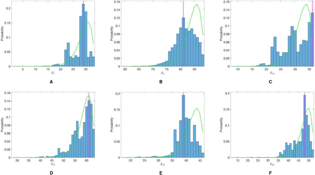
Posterior distributions of the unobserved infection times of a selection of VL cases with known onset times (blue histograms), with prior distributions (green lines) and modes (magenta lines).

• Download figure
• Open in new tab

Fig. S14.

Inferred transmission tree in part of the south-east cluster of villages at different stages of the epidemic — (A) Dec 2003, (B) Dec 2005, and (C) Dec 2009 — from a single sample from the joint posterior distribution of model parameters and missing data. Model parameters chosen close to the posterior mode (β = 1.9 mnth⁻¹, α = 114 m, = 5.6 × 10⁻⁴ mnth⁻¹, δ = 0.100 mnth⁻¹, p = 0.33). Dots show susceptible individuals/symptomatic cases and crosses asymptomatic individuals, and are coloured by infection state (see key). Arrows show the source of infection for each VL case infected up to that point in time and are coloured by type of infection source. GPS locations of individuals are jittered slightly so that individuals from the same household are more visible. An animated version showing all months is provided in SI movie S2.

• Download figure
• Open in new tab

Fig. S15.

Para-level annual incidence of (A) VL and (B) PKDL. Insets: distributions of annual incidences.

• Download figure
• Open in new tab

Fig. S16.

Estimated spatial transmission kernel showing decrease in infection risk with distance from an infectious individual. Transmission risk per month, βK(d), shown as a function of distance d away from a VL case (solid black line = mode, dark grey shaded region = 95% CI). Background transmission rate,, for unexplained infections also shown for comparison (dashed black line = mode, light grey shaded region = 95% CI). Inset: enlarged view of the part of the transmission kernel outside the household of the VL case.

• Download figure
• Open in new tab

Fig. S17.

Relative contributions of background transmission, asymptomatic individuals, pre-symptomatic individuals, VL cases and PKDL cases to the total risk of new infections.

• Download figure
• Open in new tab

Fig. S18.

Number of secondary infections generated by (A) each VL case and (B) each PKDL case. Dots show mean reproduction number, bars show 95% CI (2.5–97.5% quantile).

• Download figure
• Open in new tab

Fig. S19.

(A) Distributions of mean numbers of secondary VL cases per VL case and PKDL case. (B) Relationship between mean number of secondary infections and onset-to-recovery time for VL and PKDL cases and infection-to-recovery time for asymptomatic individuals. (C) Effective reproduction number R(t) with contributions from asymptomatic individuals, VL and PKDL cases. Solid lines show medians, and shaded bands 95% CIs.

• Download figure
• Open in new tab

• Download figure
• Open in new tab

Fig. S20.

Para-level epidemic curves simulated with the individual-level spatiotemporal transmission model starting from January 2003 (by which point all but one para had had at least 1 VL case since January 2002) under normal conditions (solid grey lines) (17% of VL cases develop PKDL and 0.3% of asymptomatic individuals develop PKDL) and with complete prevention of PKDL (solid pink lines). Solid coloured lines show 100 randomly chosen simulations from 10,000 simulations (100 samples of the model parameters and initial infection statuses from the posterior distribution each simulated 100 times), solid black lines show observed incidence of VL, dashed lines show the minimums and maximums of all the simulations at each time point.

Movie S1. Animation of the evolution of the most likely transmission tree in Fig. 3 in the main text over the course of the epidemic from January 2003 (t = 13) to December 2010 (t = 108). Dots show individuals coloured by their infection state (see key). Arrows show the most likely source of infection for each case over 1000 sampled transmission trees, coloured by type of infection source and shaded according to the proportion of trees in which that individual was the most likely infector (darker shading indicating a higher proportion).

Movie S2. Animation of the transmission tree shown in Fig. S14 from a single sample from the joint posterior distribution of model parameters and missing data. Dots, crosses and arrows as in Fig. S14.