
Abstract
Medical imaging, like computed tomography (CT) and magnetic resonance imaging (MRI), holds profound value in disease diagnosis for millions worldwide. However, studies show that physician imaging orders may frequently be inappropriate (26% of cases) for the corresponding patient evaluation. Measures are necessary to mitigate patient risks in the subsequent re-imaging necessitated by physician error, including radiation exposure, additional sedation (pediatrics), and delayed treatment. To address these dangers, AIM-AI presents an unprecedented platform for automated medical imaging order selection using natural language processing and machine learning (ML). The algorithm was trained with anonymized imaging records and associated provider-input symptoms for 40,667 patients from Texas Children’s Hospital, obtained after institutional review board approval. First, the data was preprocessed using tokenization and lemmatization to extract keywords. Second, an entity-embedding ML model converted the symptoms to high-dimensional numerical vectors suitable for model comprehension, which we used to balance the dataset through k-nearest-neighbor-based synthetic sampling. Third, a Support Vector Classifier (ML model) was trained and hyper-parameter tuned using the em-bedded symptoms to predict modality (CT/MRI), contrast (with/without), and anatomical region (head, neck, etc.) for an imaging order with 93.2% accuracy on 4,704 test cases. Finally, a web application was developed to package the model, which analyzes user-input symptoms and outputs the predicted order. The implementation of this application would save the lives of millions of patients facing potentially fatal risks associated with medical imaging by reducing costs, expediting treatment, and maximizing patient health. In this way, AIM-AI paves the path to a revolutionized medical field.
1 Introduction
Magnetic Resonance Imaging (MRI) and Computed Tomography (CT) are routinely used in the diagnosis of various diseases, playing a crucial role in disease identification for millions of people worldwide [1–3]. These imaging techniques allow healthcare professionals to visualize internal struc-tures, enabling them to identify cancerous or diseased tissues, injuries, and neurological disorders. By using this information, medical professionals can carefully plan treatments to accurately address the underlying conditions.
1.1 Purpose
Although their general purpose is the same, MRI and CT scans are necessary for different diagnosis requirements. MRI is a non-radiation imaging process that utilizes the nuclear magnetic resonance phenomenon to generate images of soft tissue structures. By aligning hydrogen atoms in the body with the magnetic field and perturbing them with radio waves, the MRI scanner measures the result-ing energy release and constructs a three-dimensional representation of the tissues being examined [2–7]. In contrast, a CT scan conducts numerous X-ray projections to create detailed cross-sectional images of the body with millimeter precision[8–10]. An intramedullary tumor, for example, would require an MRI scan due to its sensitivity in detecting soft tissue abnormalities. A broken bone, however, would require a CT scan due to its ability to visualize dense structures.
1.2 Imaging
The significant growth of the medical imaging industry has increased over two-fold from $3.6 billion to $7.6 billion over a period of 7 years[11]. This growth highlights the increasing prominence of medical imaging in healthcare. However, this rapid rise is also characterized by the need for im-provements in imaging efficiency, from the initial physician encounter to the MRI/CT evaluation by the specialist. The imaging process involves numerous interactions between the patient, insurance company, physician ordering the image, and the clinic responsible for carrying out the order. As a result, the imaging process can lead to an extended patient timeline. A long process such as this in a rapidly increasing industry calls for the need for efficient and appropriate imaging. Artificial intel-ligence has proven to be necessary for CT scans for patient positioning, scan positioning, protocol selection, CT parameter selection, and image reconstruction [12].
1.3 Concerns
Imaging appropriateness has been of important concern in the effort to improve medical imaging efficiency and cost reduction. A past study showed that 26% of medical imaging orders were identified as inappropriate [13, 14]. This high proportion has four main consequences for patients. (i) Re-imaging leads to excessive radiation, which has a well-established link to cancer and other disorders [15–18]. (ii) MRI/CT scans require pediatric patients to be sedated, and repeating this can cause cardiopulmonary complications [19, 20]. (iii) The patient recovery timeline can be delayed due to the aforementioned long process of imaging having to be repeated, and for a patient with an undiagnosed yet critical condition, timing can be the difference between life and death. (iv) The increased costs of reimaging can put a financial strain on not only the patient, potentially preventing them from further treatment, but also the hospital, which could better spend those funds to help more patients[21].
Physician-based clinical decision support systems (CDS) have been demonstrated to improve the efficiency of image ordering and reduce re-imaging rates significantly [22], and artificial intelligence has a potential impact in protocol/order selection in medical CT scans specifically [8]. However, limited research is available on the effectiveness of computer-based imaging order CDS algorithms. To address this gap in the literature, we conducted a study to develop an AI algorithm with NLP that can effectively determine the most appropriate imaging order for a patient based on their clinical signs and symptoms within a clinical setting. We hypothesized that implementing a computer-interface-based CDS would enhance clinical efficiency and reduce the likelihood of the four aforementioned devastating consequences of re-imaging a patient.
2 Methods
2.1 Data Collection
Data were obtained in CSV format from the Texas Children’s Hospital Department of Pediatric Neuroradiology following IRB approval and HIPAA certification. All imaging orders were verified for accuracy and anonymized per HIPAA guidelines before their use in the study.
The dataset was composed of 40,667 entries of patient symptoms paired with the corresponding imaging order as seen in Figure 1. Exploratory data analysis [23] was then conducted to identify key features for implementation in the algorithm. The initial dataset consisted of approximately 80 neurological imaging orders but was eventually reduced to the top 8 most frequent imaging orders. The distribution of the frequency of imaging orders in Figure 2 reports CT Head without Contrast as a frequent option or ordering and MRI Pituitary with less than 1000.

Sample Data

Class Distribution
The data in Figure 1 included information on various unidentifiable patient attributes namely age, weight, and height. which were assessed for their contribution to the model’s output. It was determined that these columns would introduce unnecessary features with low predictive power due to their randomness and were therefore excluded. The average word count of the clinical signs/symptoms showed an average of 4.6 words indicating the limited information provided with each entry (Fig. 3). Three key issues were identified in the data that impacted our approach prior to algorithm implementation. First, the degree of irregularity present required the implementation of a pre-processing step prior to ML. Many rows consisted of abbreviations, irregular capitalization, incorrect spelling and grammar, and empty entries. Second, a severe data imbalance, with nearly 11,000 cases of CT Head without Contrast and just 1,000 of MRI Pituitary indicated the need for class balancing, either with under-sampling or oversampling [24]. Lastly, the most frequent word count of the symptom text rows was found to be just three, as seen in the distribution graph, indicating that each word present contributes significant meaning and that any pre-processing should be somewhat conservative (Fig. 3).

Word Count Distribution
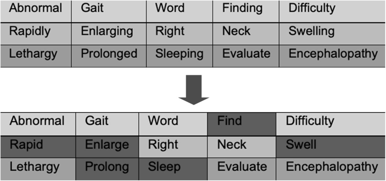
Lemmatization
2.2 Preprocessing
A three-step processing algorithm addressed these data irregularities. The initial step was to nor-malize and condense the symptom text. Our initial approach was to utilize OpenAI’s Davinci GPT-3 API [25] to ask it to extract important keywords and include similar words to the existing prompt for additional data. This approach proved to be costly and computationally expensive as it required API and tokens for purchase. The alternative was the Natural Language Toolkit (NLTK) which tokenizes each symptom row and filters through the StopWord corpus to identify stop-words [26]. As opposed to extracting important keywords, the algorithm uses the corpus to identify and extract unnecessary filler words that serve no significant meaning such as “with”, “to”, and “also”. It proved to be the most effective approach in normalizing the data and accounted for special characters and irregular syntax as seen in Figure 5. However, using the NLTK library sacrificed the ability to correct spellings, a feature that the GPT model would automatically account for.

Keyword Filtering

Entity Embedding
Following keyword filtering, word lemmatization was performed to simplify each word to its most fundamental grammatical root and maintain consistency across conjugations as seen in Fig. 5 (e.g. “flying” transformed to “fly”) [27, 28]. Lemmatization was preferred over stemming due to its higher accuracy but at the expense of computational speed [29, 30]. Without lemmatization, however, the model is introduced to more variability in words and would impact the accuracy of the model.
To facilitate ML model training, it was necessary to transform the symptom text into numerical representations [31]. The reasoning of use of an embedding model for text-to-numerical represen-tations was two-fold over the established one-hot encoding approach - the computation time is significantly increased and the dimensionality of the encoding approach of a 40,000-row dataset would magnify the complexity of the algorithm carrying out downstream tasks [32, 33]. The fo-cus went on utilizing the optimal model for entity embedding. With limitations of computational power and a limited solution timeline, the choice was dependent on the previous literature on the trade-off of accuracy to time complexity. We leveraged OpenAI’s 1.2 billion-parameter pre-trained and custom-tuned Ada embedding model [34], which uses entity embedding techniques to convert each symptom row into dense 1536-dimensional numerical vectors to convey both the definition and context of the input (Fig. 5). The model architecture first embeds each word into a vector and then uses multi-head self-attention transformer layers to understand and generate relationships between the words. Word2Vec, a prospective alternative embedding algorithm, was not preferred in this use case due to possible words un-encountered in the pre-trained base embedding and presence of pairs of structurally similar words but different definitions [35].
Referenced before, Figure 2 magnifies the severe class imbalance present in the dataset. Training an ML model with imbalanced data with a majority-minority ratio of approximately 15:1 is sub-optimal to maximize accuracy as much as possible. To combat this, a synthetic sampling algorithm assisted in balancing the dataset following entity embedding. We utilized a synthetic minority oversampling technique (SMOTE) k-nearest-neighbor algorithm [36], which is designed to construct new points close to existing ones in high-dimensional feature space, thereby increasing the number of samples of the minority class. A sample point is paired with a neighbor and the difference between the points is multiplied by a random number which then creates a new point in between the two existing points. SMOTE has also been proven to work well in high-dimensional datasets [37]. Each of the minority classes was oversampled to match the count of the majority class (CT Head without Contrast). SMOTE increased the sample size from 40,667 to approximately 90,000 rows and was used to train the final ML model (Fig. 7). Basic minority oversampling and majority undersampling techniques were also tested, however, the SMOTE algorithm was found to be more effective at increasing the variety of data present in a limited dataset [38]. By generating synthetic data points, the algorithm was able to maintain the underlying structure of the data while eliminating the problem of class imbalance.

Synthetic Sampling
2.3 Machine Learning
Selecting a model required a rigorous experimental design, training, and testing of three distinct supervised alternatives on the same dataset with default model parameters. This approach allowed for a reliable assessment of the most effective model for accurate classification. Specifically, the models tested were XGBoost, which utilizes gradient boosting and decision trees to iteratively learn from residuals and minimize loss; Random Forest, an ensemble learning method that constructs multiple decision trees to aggregate their outputs and improve prediction accuracy; and Support Vector Machine (SVM), a robust classification algorithm that identifies a hyperplane to optimally separate data points of different classes in a high-dimensional feature space through a maximum margin function. Evaluation of all three models proved the Support Vector Classifier to be the best for the dataset as seen in Figure 8. The reasoning of the model was two-fold. (i) It was critical to prevent the model’s overfitting, a problem commonly associated with high-dimensional data SVMs [39, 40]. The SVM is comparatively better than regression algorithms and other classifiers in preventing overfitting in high-dimensional space leading to overall improved performance in high-dimensional datasets [41, 42]. (ii) SVM classification models being resistant to noise [40]. This is important in medical NLP where abbreviations and other anomalies are included in the history [43].

Model Comparisons
The straight line for the boundaries of each classification region in a linear SVM classifier is defined as:
 where
where  is [β0, β1] which is perpendicular to the hyperplane and
  is [x1, x2] is the point on the straight line.
Equation 1 can be generalized to:
 or
or
 Xi is defined as the vector to display all features of index i. With
  describing the positive class and
  describing the negative class. The support vectors can be defined as
 Provided that Yi is a vector containing values -1 and +1. Equation 4 can be generalized into
 The width of the margin is then defined as
 or
or
 And to maximize Equation 7, the model must minimize
 Lagrangian Transform then optimizes Equation 8 with constraints of Equation 5.
 Since
Since

 Which leads to
 From here, we see that the SVC depends on
  .
.
Each model was trained on the pre-processed data and was validated on a 4704(5%) randomly sampled test case set with accuracy metrics. Accuracy, in terms of True Positive(TP), True Nega-tive(TN), False Positive(FP), and False Negative(FN).
 After selecting a model, the support vector machine further optimized the model’s performance through GridSearchCV which further optimized the model’s performance by conducting tuning of six model parameters using GridSearchCV. The GridSearchCV starts with random hyperparameters and slowly optimized the model through a trial-and-error method. The perfect model is met when there is a balance between underfitting and overfitting, therefore increasing the metrics of the model [44–46]. The parameters that were optimized were Kernel, C, Gamma, and Train-Test split. A low-degree polynomial kernel is optimal in NLP situations [47, 48].
With x and y reprinting the input vectors, φ(x) and φ(y) representing the mapping functions, the polynomial kernel works as follows:

3 Results
The models were successfully trained and tested on the preprocessed dataset. Notably, the SVM exhibited the highest accuracy of 91.5% on a randomly sampled test case set of 4704 from the original data, outperforming the other models (see Fig. 8 for model accuracies). The GridSearchCV then increased the SVM accuracy by 1.7% to 93.2
Precision, recall, and F1 scores painted a more detailed picture of the intricacies of the model (Fig. 9), and each can be defined in terms of the number of true positive (TP), true negative (TN), false positive (FP), and false negative (FN) cases for the given classification in the test set.

Classification Report
Precision represents the proportion of retrieved positive cases that were relevant and is calculated as:
 Recall represents the proportion of relevant positive cases that were retrieved by the model and is calculated as:
 The F1 score is the harmonic mean of precision and recall.
 MRI Pituitary WO/W Contrast had the highest scores of all three metrics at 0.97, 0.99, and 0.98 respectively, suggesting confidence with this class. MRI Brain WO/W Contrast had the lowest scores of all three metrics at 0.84, 0.72, and 0.77 respectively, suggesting that this class may be highly similar to another. However, the average of all individual class metrics came out to be 0.92, 0.92, and 0.92 respectively, confirming the model’s overall accuracy.
The heatmap in Fig. 10 assists in visualizing class-specific performance as well. Similarly, the receiver operating characteristic (ROC) curves seen in Fig. 11 demonstrate a strong tradeoff between true and false positives. An area under the curve (AUC) close to 1 for each class indicates an accurate model. The model achieved near-perfect AUC values for three classes: CT Soft Tissue Neck With Contrast, CT Maxillofacial Without Contrast, and MRI Pituitary WO/W Contrast. These findings are consistent with the high metrics observed for the classes above in Fig. 9.

Heatmap

ROC Curves
To properly visualize the internal workings of the algorithm, the 1536-dimensional data was compressed into a two-dimensional array through a t-distributed stochastic embedding (TSNE) network. tSNE is a dimensionality reduction technique that embeds the 1536 features present into two or three dimensions for visualization. Each individual point represents a case, all of which can be observed to be clustered based on class.
In order to carry out the tSNE algorithm, the high-dimensional Euclidean distances between any two datapoints xi and xj is first found in the form of conditional probabilities, which represent the similarity between the points. The conditional probability pj|i that xj is near xi is calculated using a Gaussian distribution centered at xi with a standard deviation of σi and is defined as:
 The high-dimensional joint probability distribution can then be calculated as:
 Next, a second joint probability distribution is constructed in low-dimensional space. The con-ditional probability qij representing the similarity of any two points yi and yj is calculated with a t-distribution:
 Finally, the deviation between the low- and high-dimensional data point distributions must be minimized, which can be done using the Kullback-Leiber (KL) divergence. The KL divergence for distributions P and Q in space χ is defined as:
 Gradient descent is employed to iteratively modify the low-dimensional data to best match the high-dimensional data. To do this, the cost function C must be minimized. C represents the KL divergence of the joint probability distributions P, from the high-dimensional data, and Q, from the low-dimensional data and is defined as:
 The results are shown in Fig. 12.

tSNE 2D
Hyperplanes were then drawn to view the classification boundaries of the SVM (Fig. 13). Due to its large compression ratio (1536/2 = 768), many features were most likely lost, so the classification in a two-dimensional space is not entirely representative of the 1536-dimensional hyperspace but does serve as a rough model. The poor classification of points seen in the MRI Brain WO/W Contrast class in Fig. 13 is consistent with the relatively low class-specific metrics observed in the classification report in Fig. 9.

Decision Boundary Plot
The accuracy of the SVM model does appear to be significantly higher than the physician accu-racy of 74.3%, but a one-way two proportion z-test confirmed that there was a statistically significant difference in the physician imaging order accuracy of 74.3% and SVM model imaging order accuracy of 93.2% (p < 0.0001). In the context of the 100 million MRI/CT scans done annually, an increase of 18.9% in imaging accuracy can prevent 18.9 million patients from the effects of excessive imaging.
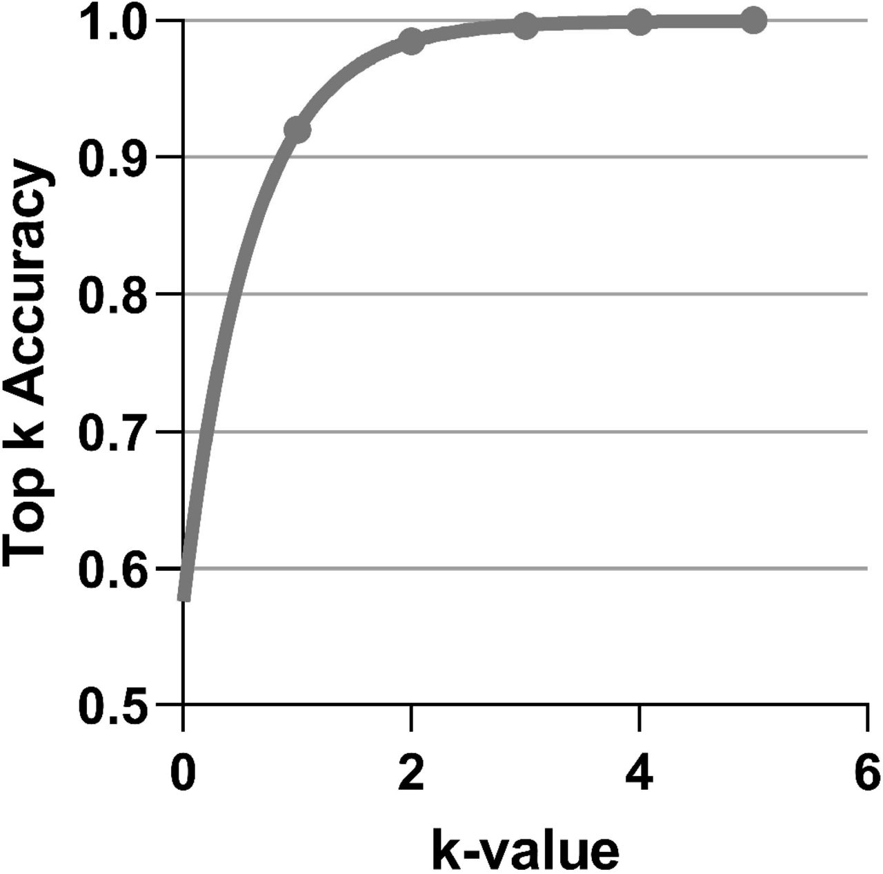
In order to maximize the efficacy of the ML model and provide a more realistic clinical tool, a probability-based prediction system was implemented that provides the probability of each class fitting the input, rather than outputting a single classification. The algorithm, by default, offers the top three highest-probability class results with a 100% chance that the class labeled as correct will be present in the top three (Fig. 14).

Top K Accuracy
4 Discussion
This algorithm proves the effectiveness of an automated approach to mitigating existing risks of incorrect imaging order selection by physicians. However, a raw algorithm is impractical for a practicing physician, who requires a straightforward user interface. After the study, the model was packaged into a web application that receives free-text symptom input and uses it to output the predicted imaging order with a confidence score. This application acts as a clinical decision support tool, allowing physicians an additional verification step to produce a combined imaging order selection accuracy of over 93%.
A notable use for this tool is in emergency settings. Rather than requiring a physician to evaluate a patient both before and after receiving imaging, the application would reduce strain on the physician by eliminating any need for them to see the patient until after imaging and diagnostics have been completed, which would maximize hospital efficiency.[49] Patients could realistically be rapidly evaluated, receive an imaging order from the tool, undergo imaging, and have the results read in a short time frame, which would improve their treatment outlook.
The widespread implementation of this algorithm holds potential for several positive outcomes as a result of decreased re-imaging due to more accurate imaging order selection.[22] First, excessive radiation brought by several imaging methods, namely CT scans, would be mitigated. Presently, radiation, which is significantly carcinogenic, can be presented in unnecessarily high dosage when imaging must be carried out multiple times.[15, 50] With improved imaging order selection, fewer cases of re-imaging would reduce radiation exposure to a minimal level.
The algorithm would, furthermore, eliminate repeated sedation in patients, reducing the potential for complications. Pediatric patients, as well as adults with certain conditions such as claustropho-bia, require sedation when being imaged, but such practices pose risks of complications for those patients.[51] By minimizing the number of instances of sedation, the algorithm will maximize patient health outcomes.
Reducing re-imaging would also expedite patient treatment timelines. The process of imaging, including carrying out the imaging, reading results, and conveying the outcome to the patient, is time-consuming, and for patients with unknown critical conditions, repeating these steps due to physician imaging order error can be life-threatening. Without re-imaging, the duration of diagnostic testing is lessened for improved treatment options. [52].
A final advantage is the reduction of costs for both the hospital and patient that is brought by more precise imaging ordering. [53] Hospital systems currently spending millions to carry out imaging orders would see significant drops in spending with the implementation of this algorithm.[11] By instead applying these funds to causes such as research, medical facilities could see a growth in innovation and potentially revolutionary treatment breakthroughs.
Despite the numerous benefits of this tool, there exist several avenues for further development that would optimize its effectiveness. Enhancement of this algorithm’s accuracy metrics will most importantly require the incorporation of more training data. The present data includes just one feature (clinical symptoms) and originates from a single hospital institution. Incorporating vital signs, laboratory orders, family history, and clinical guidelines from multiple institutions in the model could certainly see an additional 4-5% accuracy increase.
The present dataset also is limited to neurological imaging orders; however, due to the gener-alizability of the algorithm, this can be easily diversified.[54] Because this model does not need to be adapted to specific features of the dataset, any additional, similarly-structured data (free-text input + class-based output) could be used in training to also produce high accuracy rates. In this way, with datasets for other body systems, such as gastrointestinal imaging orders, the scope of the model could quickly be grown to fit any medical specialty, and the application’s online nature will allow for real-time remote updates to the platform.
5 Conclusion
This algorithm has significant potential to be truly revolutionary for the millions of patients facing incorrect imaging orders in the United States. Beyond this, scaling the application to the rest of the world would impact millions more by reducing costs through fewer scans, expediting treatment through more efficient diagnosis, and maximizing patient health through reduced radiation and se-dation. This tool will certainly be critical for a more efficient healthcare system and groundbreaking to the medical field as a whole.
Data Availability
The data provided in the manuscript is a private dataset from Texas Childrens Hospital not available for request.
Author Contributions
All authors contributed equally to the writing of the manuscript.
Conflicts of Interest
The authors have not declared any conflicts of interest.
Acknowledgements
The authors would like to thank Texas Children’s Hospital for providing the project dataset and offering project feedback from a medical perspective.
Footnotes
Moved the figures to the end of the manuscript, and added a senior author to the paper that is helping with reviewing and publication, and fixed some figure referencing issues.
References


