
Abstract
Clinical classification is essential for estimating disease prevalence in a population but is difficult, often requiring complex investigations. The widespread availability of population level genetic data makes novel genetic stratification techniques a highly attractive alternative. We propose a generalizable mathematical framework for determining the prevalence of a disease within a population using genetic risk scores. We compare and evaluate methods based on the means of the genetic risk scores’ distributions; the Earth Mover’s Distance between distributions; a linear combination of kernel density estimates of distributions; and an Excess method. We assess the impact on estimates resulting from the population size and proportion of cases to non-cases. Using less discriminative genetic risk scores still results in robust estimates of proportion. Genetic stratification techniques provide exciting research tools enabling unbiased insights into disease prevalence and clinical characteristics unhampered by clinical classification criteria.
Introduction
The development and refinement of polygenic analysis techniques is greatly increasing our understanding of many diseases. Using polygenic risk has allowed insights into disease etiology and through Mendelian randomization evaluation of causality 1. Clinically, capturing polygenic susceptibility through Genetic Risk Scores (GRS) can be used to determine individuals at the highest risk of a disease 2-4. This paper concentrates on an innovative use of polygenic risk to genetically stratify a population into those with and without a certain disease. Currently estimates of prevalence require disease specific investigations to facilitate clinical classification. Given the increasing availability of population level genetic data, novel polygenic estimates of disease prevalence, which negate the need for biochemical tests, are an extremely attractive alternative.
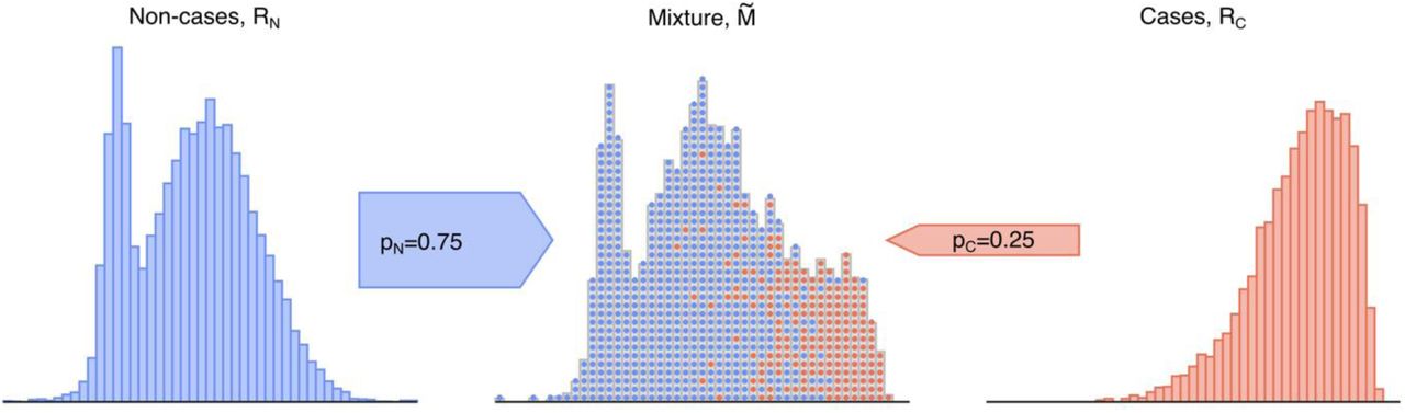
The basis of genetically determining disease prevalence is simply that the distribution of a specific disease GRS within a population will reflect the mixture of genetic risk scores of those with the disease (cases) and those without (non-cases). This mixture GRS distribution will lie between reference populations of cases and non-cases and will reflect the relative proportion of cases to non-cases (Fig. 1). The location of the mixture population’s GRS distribution in comparison to the GRS distribution of known cases and non-cases allows the respective proportion of each group to be determined and provides a genetic-based estimate of disease prevalence. Furthermore, using the genetically calculated proportion of a disease within a population allows the additional benefit of associated clinical features of the genetically defined disease cohort to be determined. It is worth emphasising that in almost all polygenic risk situations, even those at the highest genetic risk are unlikely to develop the relevant disease and therefore this concept is not valid at an individual level. Nonetheless, at a population level the average genetic risk score will be higher in a cohort with disease versus those without.

Illustration of a mixture population drawn from two reference populations. This emulates the real-world scenario of a population composed solely of individuals drawn from each subpopulation of non-cases (RN, blue) and cases (RC, red). Data are sampled with replacement from the two depicted reference populations to generate a mixture  population of a particular sample size and proportion, which possesses features of both reference populations. Figure generated using artificial data.
To date only one method of genetic stratification has been used to evaluate one polygenic disease. Thomas et al. 5 showed a genetic excess of type 1 diabetes within the UK biobank. If the concept of polygenic stratification is to be widely utilized, assessment of a number of approaches and factors impacting on accuracy are required. This paper assesses, through modelling and bootstrap techniques, the general utility of polygenic stratification as a tool for determining disease prevalence. Through simulated scenarios and real-world data, we evaluate different mathematical techniques for determining disease prevalence based on the GRS distribution within a population. We analyse the impact of the mixture population size and proportional makeup as well as the discriminative ability of the GRS being utilised. Finally, we apply the proposed framework in the context of identifying the prevalence of undiagnosed coeliac disease within a cohort adhering to a gluten-free diet.
Results
We present three methods developed to estimate the proportions of cases and non-cases in an unknown mixture population using GRS distributions and compare them with the published Excess approach 5. The methods’ performance characteristics are evaluated over clinically relevant parameter ranges using genetic risk scores for synthetic data, type 1 diabetes, type 2 diabetes and coeliac disease. In particular, for each algorithm we characterise the impact of sample size, proportion of cases and non-cases within the population and the discriminative ability of the GRS on estimation accuracy (defined as deviation from the true proportion). Finally, we present a worked example estimating the amount of undiagnosed coeliac disease within a population adhering to a gluten-free diet.
Methods Summary
In each method, two populations consisting of the genetic risk scores of individuals with and without a particular polygenic disease were taken as references, denoted RC (the reference population of cases) and RN (the reference population of non-cases). The proportions of individuals from these reference populations (denoted pC and pN respectively) who comprise an unknown mixture population  were estimated from characteristics of the reference populations. When only one proportion is mentioned, this is pC (i.e. relative to the Reference Population of cases, RC), unless otherwise stated. The population characteristics used are dependent upon the particular method employed as illustrated in Fig. 2 and are detailed below.

Illustration of the four proportion estimation methods. Each method uses different characteristics of the mixture and reference populations to estimate the proportion of constituents of the mixture population (pC and pN). The Excess method (A) considers the number of cases above the mixture median in excess of those expected in a pure disease reference population. The Means method (B) uses the normalised difference of the mixture population’s mean and the two reference populations’ means. The earth mover’s distance method C) uses the weighted costs of transforming the mixture distribution into the reference populations. The Kernel density estimation method (D) fits smoothed templates to each of the reference populations and then fits a weighted sum of these templates to the mixture population, adjusting the amplitudes of each with the Levenberg–Marquardt algorithm. Figure generated using artificial data.
Throughout this paper we assume that the unknown mixture population is composed solely of the samples that come from the two reference populations (blue and red dots in Fig. 1). In practice, this means that pN prevalence of non-cases and pC prevalence of cases sum to one, pN + pC = 1, and so accordingly, the proportion of non-cases was calculated as: pN = 1 − pC. Nonetheless, the presented Earth Mover’s Distance (EMD) and Kernel Density Estimation (KDE) methods make it possible to check if this assumption is satisfied. We revisit details of such checks in the discussion and supplementary information.
The Excess method
This estimates the proportion from the number of excess disease cases above the mixture population’s median score compared to the equal numbers expected in a pure control population (Fig.2A). We illustrate the method as introduced in 5.
The Means method
This compares the mean genetic risk score of the mixture population to the means of the two reference populations and estimates the mixture proportion according to the normalised difference between the two (Fig.2B).
The Earth Mover’s Distance (EMD) method
This uses the weighted cost of transforming the mixture population into each reference population (more formally, the integral of the difference between the cumulative density functions, i.e. the area between the curves). The method allows pN and pC to be computed independently (Fig. 2C) and so provides a way to validate the assumption that the mixture is composed solely of the samples from the two reference populations, pN + pC = 1; if the sum is significantly different from 1, then the assumption is not satisfied. In this study we use the mean of the two estimates for  and
and  as the estimate of the pC. We further note that whenever
  the averaged pC will be overestimating small proportions and underestimating large proportions.
The Kernel Density Estimation (KDE) method
This method fits a smoothed template to each reference population (by convolving each sample with a Gaussian kernel) and builds a model of the mixture as a weighted sum of these two templates. The method then adjusts the proportion of these templates with the Levenberg– Marquardt (damped least squares) algorithm until the sum optimally fits the mixture distribution (Fig.2D), noting that the algorithm could find one of potentially several local minima. In other words, the method finds (one of) the linear (convex) combination of the distributions of the reference populations that best fits the mixture distribution.
Effect of mixture size and constituent population’s proportional contribution on method performance
We start by using the type 1 diabetes genetic risk scores (T1DGRS) to evaluate the performance of all four methods on carefully constructed example mixtures. To simulate a range of real-world scenarios, we constructed these artificial distributions by randomly sampling genetic risk scores from the reference populations of cases (RC) and non-cases (RN) in specified proportions and total mixture sizes (Fig. 3). We find that the Means, KDE and EMD methods perform well in estimating prevalence. The Excess method demonstrates reduced performance despite significant bias correction, this is further emphasised by Supplementary Fig. 1. In Fig. 3 we see that the precision of the proportion estimates increases with sample size. Larger sample sizes can be seen to represent the characteristics of the reference distributions more accurately, allowing the methods to more reliably estimate the true proportions.

A comparison of the 4 methods prevalence estimates and confidence intervals for varying proportion of disease and for 3 sample sizes. Mixture distributions of controls and Type 1 diabetes patients from WTCCC 6 were constructed with  (shown in blue, grey and red respectively) and n = {500, 1000, 5000}. (Left column) The constructed mixture distributions and reference distributions (RC, shaded red and RN, shaded blue) from which they were constructed. (Right column) Prevalence pC estimates (bullseye) obtain by each of the 4 methods for varying
  and sample size, n (rows). Each estimated pC value is shown together with violin plot illustrating the distribution of the 100,000 estimates of prevalence
  in the bootstrap samples and with confidence intervals (α = 0. 05; horizontal line with vertical bars at the ends). Dashed vertical lines indicate reference prevalence values
  . In all the cases, for the Excess method we observe a large offset between the violin plots and the pC value and its confidence interval. This offset is a result of the systematic bias of the Excess method. Employed bootstrap methodology allows the correction of such bias. Calculations were based on the following participants: cases WTCCC type 1 diabetes, non-cases WTCCC Type 2 diabetes.
More detailed analysis of the continual effect of mixture size and proportion on accuracy and rate of convergence to true prevalence of the estimates is presented as heat maps in Supplementary Fig. 1. This allowed direct comparison of the effects of sampling from reference distributions for all four methodologies. In all cases accuracy reduces at extremes of proportion, (tending to underestimate high proportions and overestimate low proportions), least significantly with the Means and KDE methods.
Effect of genetic risk score discriminative ability
Next we investigate the dependence of estimates on the discriminative ability of the GRS, Fig 4. To carry out this investigation we evaluate the impact of decreasing the discriminative ability of the GRS on the accuracy of estimates across two different mixture sizes (n = 1,000 and n = 5,000) using all the methods. To this end we create artificial genetic risk scores with an area under the ROC curve (AUC) varying from completely non-discriminative (AUC = 0.5) to completely discriminative (AUC = 1), shown in Fig. 4B. Figure 4 shows that decreasing AUC leads to a reduction in precision (reduced accuracy and increased CI). Increasing the mixture size from 1,000 to 5,000 improves accuracy across all ranges of AUC. With a mixture size of 5,000 or above the Means, EMD and KDE methods perform well but the EMD and KDE allow more robust estimates at extremely low levels of genetic discrimination as defined by AUC. Fig. 4A shows that regardless of the mixture size, the Excess method is practically unusable for any but the highest AUC. The paradoxically comparable performance of the Excess method in Fig. 3 is a consequence of the high AUC of the T1DGRS (0.88) and the strong asymmetry of the reference populations.

A comparison of the four methods using an artificial genetic risk score with increasing discriminative ability as measured by AUC, from AUC = 0.5 (no discriminative ability) through to AUC = 1, (complete differentiation). The estimated proportion with confidence intervals for each of the methods (Excess, Means, EMD, KDE) are shown using mixture populations with sample size, n = {1000, 5000}. This figure is generated using artificial data: N(μ,σ) is a normal distribution with mean μ and standard deviation σ and  is an equal mixture of the two normal distributions
  .
.
The effect of reduced discrimination on estimation accuracy across a continuum of proportions and mixture sizes is presented in Supplementary Fig. 1 which shows heat maps of the estimation accuracy for the less discriminative T2DGRS (AUC = 0.61) as a comparison to when using the T1DGRS (AUC = 0.88) (Supplementary Fig. 2). Supplementary Fig. 2 also highlights that the extremes of proportion, where the methods display reduced accuracy, are increased using a less discriminative GRS.
Clinical example
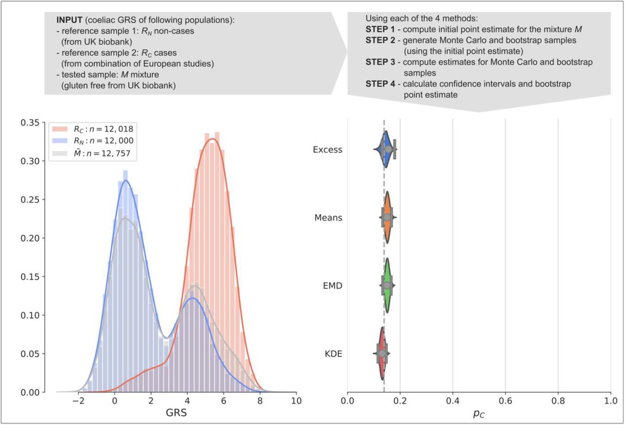
Finally, we illustrate a worked example asking the question of how much undiagnosed coeliac disease is present within a population adhering to a gluten-free diet (Fig. 5) using a coeliac disease GRS (CDGRS). Whilst people observe a gluten-free diet for a number of reasons, it is possible that without getting a formal diagnosis people with undiagnosed coeliac disease eliminated gluten from their diet using trial and error to alleviate abdominal symptoms. For each method we: 1.) compute a point-estimate of prevalence 2.) use modelled mixtures and bootstrapping to 3.) find confidence intervals and bootstrapped point estimates. All methodologies provide estimates of the proportion of individuals with coeliac disease with their 95% CIs (square brackets) shown: Excess = 15.5% [13.1%, 17.9%], Means = 15.0% [13.4%, 16.7%], EMD = 15.0% [13.4%, 16.6%], KDE = 13.2% [11.6%, 14.7%]. The 13.9% prevalence of the coeliac disease was calculated from reported cases in the UK biobank. Our results suggest an absence of undiagnosed coeliac disease in the 86.1% of patients adhering to a gluten free diet and not known to have the condition.

Coeliac disease dataset worked example. A comparison of the four methods applied to a gluten-free cohort from the UK biobank (mixture population  ). The reference and the mixture distributions are plotted on the left (RC, shaded red, RN, shaded blue,
  , shaded grey, respectively). Estimated values of prevalence pC and 95% confidence intervals (grey dots and lines with bars at the ends) are plotted on the right showing estimates of Excess = 15.5%, Means = 15.0%, EMD = 15.0%, KDE = 13.2%. The violin plots show the distribution of the 100,000 estimates of prevalence
  in the bootstrap samples. The proportion of participants adhering to a gluten-free diet and reporting coeliac disease is shown as a dashed vertical line. Calculations were based on the following participants: non-cases UK Biobank, cases coeliac disease reference cohort, mixture self-reported gluten-free diet UK Biobank.
Discussion
We present analysis of a novel approach to disease classification based on genetic predisposition. Head-to-head evaluation of four methods including the original Excess methodology published by Thomas et al. 5 was performed. The presented examples illustrate the accuracy of estimates from each method across a range of different scenarios. We combined Monte Carlo sampling 7 and bootstrap 8 methods to quantify estimation uncertainty and compute realistic confidence intervals.
Distribution of genetic risk scores can be used to estimate population prevalence
Our results show that robust estimates of prevalence are possible using differences in distributions of genetic risk scores between a population of cases and non-cases. Our methods build on the previously published genetic stratification by Thomas et al. 5. This novel concept is important, as when coupled to the ever-increasing availability of large population level genetic datasets, it allows fresh insights into disease epidemiology without requiring extensive investigations. The permanence associated with genetic risk makes these methods potentially very powerful tools for researchers and enables accurate evaluation where cases are difficult to differentiate clinically.
Mixture population size and proportional makeup is important
Precision around estimates improved with increasing population size, whilst proportional makeup of the mixture, away from extremes, had little impact. Extremes of mixture size and proportional make up had a marked impact on the accuracy of estimates. The explanation for this is that sufficient numbers of individuals are required for the mixture to robustly represent the true (population) distributions of cases and non-cases. To ensure optimum sample size we recommend initially generating accuracy heat maps using reference populations in order to determine (on average) the minimum proportions and mixture sizes that can be evaluated before the real-data sample is analysed. This can then guide optimisation of mixture enrichment where the clinical criteria used to select populations can be pragmatically altered to increase disease proportion and avoid extremes of proportion where estimates are unreliable. For example, to increase the proportion of type 1 diabetes within a cohort with diabetes, the mixture population could be restricted to include only insulin treated diabetes. Mixture enrichment will inevitably be to the detriment of mixture size and therefore some reduction in confidence around estimates, but this will be outweighed by these being clinically meaningful.
Applicable to scenarios with decreased genetic differentiation
Whilst precision (improved accuracy and decreased variability) is higher when utilising a more discriminative GRS measured by AUC, we show that clinically meaningful estimates can still be drawn with less discriminative GRS. Precision is again increased by increasing mixture size and using the EMD and KDE methods. This is because the EMD and KDE are based on the entire shape of the distributions (incorporating all data) and not on their individual features (e.g. summary statistics such as the mean).
Different methods have different advantages
In most settings the best approaches are the Means, EMD and KDE methods. The overall performance of these three methods is comparable across different parameters (mixture size, mixture proportional makeup and GRS AUC). At extreme proportions the Means and KDE methods exhibit smaller deviations from the true proportion  than the EMD method. A key advantage of the Means method is that it is very straightforward to apply, allowing rapid evaluation of disease prevalence within a cohort. Alternatively, the EMD and KDE methods allow increased precision when utilising less discriminative genetic risk scores. Furthermore, the KDE and EMD methods could be used to test the assumption that the mixture is only composed of two populations.
As noted in the original article by Thomas et al. 5 the Excess method inherently underestimates the proportion of cases because typically both reference populations have values below the median value of RN, Whilst this inherent inaccuracy can to a certain degree be negated using bias correction, as described in the methods and performed throughout the manuscript, it still impacts on estimates, particularly the more the reference populations overlap as evidenced by reducing AUC (as shown in Fig. 4). Taking distinct approaches, the new methods eliminate this inaccuracy and even with decreasing genetic discrimination these are still interpretable, reflecting the improved generalizability of these methods. We note that the Excess method could be modified to improve its accuracy (e.g. by choosing another quantile than the median) but these changes would require case-by-case fine-tuning and at best achieve equivalence to the alternative methods.
Utility of using polygenic approaches to estimate prevalence within a group Prevalence
We highlight the clinical utility of the presented concept with a clinical question around coeliac disease. Exclusion of gluten from the diet is a treatment for coeliac disease. Coeliac disease can present with non-specific abdominal symptoms and diagnosis is often difficult 9. We show that it is possible to determine if there is any undiagnosed coeliac disease within a cohort adhering to a gluten-free diet using our methods. This question would be unanswerable using the traditional clinical approach of endoscopy to confirm coeliac disease as once observing a gluten-free diet findings are often normal 9. We estimated the proportion of those reporting a gluten-free diet within biobank using the coeliac disease GRS and then compared this against all those reporting a diagnosis of coeliac disease in the same gluten-free cohort. The genetic estimates and those with a reported diagnosis of coeliac disease were comparable, suggesting that there is no undiagnosed coeliac disease within this gluten-free population. Whilst this finding is not unexpected it could not be robustly shown before and highlights the general applicability of the proposed framework to answer novel and difficult to answer questions.
Defining clinical characteristics of a genetically defined subgroup
A further advantage of the proposed methodologies over traditional clinical classification arises from the fact that clinical characteristics are not used to define cases. It is therefore possible to estimate both binary and continuous clinical characteristics of the genetically defined disease group within the mixture population. Using BMI as an example:
Where pN and pC represent the estimated proportions and  and
and  represent the mean BMI of each of the non-cases, mixture and cases (disease) groups respectively. This approach was used in 5 to show rates of Diabetic Ketoacidosis to be the same in type 1 diabetes diagnosed above and below 30 years of age. We note that all the same limitations of the means method apply. The EMD and KDE methods could allow for reconstruction of the full distribution of the clinical characteristic, however evaluation of this approach is beyond the scope of this study.
Testing of proposed clinical discriminators
Another utility of these genetic discrimination techniques is to test the performance of clinical classification criteria and allow more precise stratification of a population. Whilst the increasing availability of population datasets generated from routinely collected data allows large scale population analysis, robust classification can become more difficult leading to bias which is difficult to quantify 10. Treating the clinically defined cohort as a mixture would allow rapid estimation of the proportion correctly and incorrectly classified within the cohort, thus allowing for bias adjustment and optimisation of classification criteria.
Limitations
All methods work best away from extremes of proportion (or prevalence) values. This is most noticeable in the EMD method, because in these cases the sum of the EMD estimates of prevalence is smaller than one,  . This also means that for small proportions it is practically impossible to independently confirm that the mixture does not contain samples from other populations.
The use of genetic data in the context of genetic stratification also means certain assumptions must hold true for the estimates to be valid. The same assumptions required for Mendelian randomisation 1,11 should be met here, however additional assumptions also need to be satisfied. The first of these is the retained equivalence assumption which states that cases and non-cases in the mixture reflect the respective reference populations. This is particularly important when studying different geographical populations where allele frequencies may vary, leading to an alteration in genetic risk scores across the cohorts. Ensuring this assumption is met requires detailed assessment of the cohort as well as the selection criteria of the reference populations and mixture population to ensure equivalence. Where possible as a further validation of equivalence, comparison of a control group GRS taken from the same population the mixture is derived from against the reference control group GRS should be undertaken to ensure similarity.
The second assumption is that the mixture consists of only the two genetic reference populations such that pC + pN = 1. Both, the EMD and KDE methods provide a way to check if this mixture assumption is satisfied. In the case of the EMD method we could use the independent estimates of pN and pC to check how much their sum deviates from 1. For the KDE method, the validation could be based on the residuals of the least-square fitting procedure. To check if the deviation from pC + pN = 1 is significant we again suggest the use of bootstrap methodology. We present some details and an example of such checks in the supplementary information, however detailed analysis of this aspect of the proposed methodology is beyond the scope of this paper.
Conclusion
We demonstrate novel approaches that use population distributions of genetic risk scores to estimate disease prevalence. We show that the proposed Means, EMD and KDE approaches perform similarly across different mixture populations, with robust estimates possible even when using GRS with reduced discriminative ability. Utilising these concepts will allow researchers to gain novel unbiased insights into polygenic disease prevalence and clinical characteristics, unhampered by clinical classification criteria.
Online methods
Participants
Type 1 diabetes cases
Cases (n=1,963) were taken from the Wellcome Trust Case Control Consortium 6. The WTCCC T1D patients all received a clinical diagnosis of T1D at <17 years of age and were treated with insulin from the time of diagnosis.
Type 2 diabetes cases
Cases (n=1,924) were taken from the Wellcome Trust Case Control Consortium 6. The WTCCC T2D patients all received a clinical diagnosis of T2D.
Coeliac disease reference cases
Cases (n=12,018) Cases consisted of those from a combination of European studies. Cases were diagnosed as previously described 12.
Coeliac non-cases
Non-cases (n=12,000) a sample was randomly selected from those within the UK biobank (total n= 366,326) defined as unrelated individuals of white European descent without a diagnosis of coeliac disease and not reporting a gluten-free diet.
Gluten-free diet
Gluten-free cases (n=12,757) were taken from unrelated individuals of white European descent in the UK biobank reporting adherence to a gluten-free diet.
Reported coeliac cases in biobank
Coeliac disease cases (n=1,772) were defined based on self-reported questionnaire answers and/or an ICD10 record from hospital episode statistics data.
Calculating genetic risk scores
T1DGRS
The T1DGRS was generated using published variants known to be associated with risk of T1D. All variants were present in the UK Biobank imputed genotype data. We followed the method as previously described 2 using tag variants rs2187668 and rs7454108 to determine HLA DR haplotype and ascertain the HLA-haplotype component of each individual’s score 13. This was added to the score of the remaining variants, generated by summing the effective allele dosage of each variant multiplied by the natural log (ln) of the odds ratio.
T2DGRS
The T2DGRS was generated using published variants known to be associated with risk of T2D 14. We generated a 77 SNP T2D-GRS in both the WTCCC cohort and UK Biobank consisting of variants present in both data sets and with high imputation quality (R2>0.4). The score was generated by summing the effective allele dosage of each variant multiplied by the natural log (ln) of the odds ratio.
CDGRS
The 46 SNP coeliac GRS was generated using published variants known to be associated with risk of Coeliac disease 15, 12, 16. The log-additive CDGRS was generated using a weight as the natural log of corresponding odds ratios. For each included genotype at the DQ locus, the odds ratio was derived from a previously described case-control dataset 12. For each non-HLA locus, odds ratios from existing literature were used, and each weight was multiplied by individual risk allele dosage.
Excess method
Following on from previous work 5, the Excess method calculates the reference proportions in a mixture population according to the difference in expected numbers either side of the reference population’s median. The reference median in question was taken to be the closest to the mixture population’s median. The proportion was then calculated according to:  , where m is the median of the reference population, n is the size of the mixture population and x is an individual participant in the mixture population, hence #{x > m} represents the number of cases above the median and #{x ≤ m} represents the number of cases below the median.
Means method
The mean genetic risk scores were computed for each of the two reference populations and the mixture population. The proportions of the two reference populations were then calculated according to the normalised difference of the mixture population’s mean  and the means of the two reference populations (
 and
and  ):
):  .
.
Earth Mover’s Distance (EMD) method
Intuitively, the Earth Mover’s Distance (EMD) is the minimal cost of work required to transform one ‘pile of earth’ into another; with each ‘pile of earth’ representing a probability distribution. Mathematically, the (EMD) is a Wasserstein distance and has been widely used in computer and data sciences 17,18. For univariate probability distributions, the EMD has the following closed form formula 19;
Here, PDFC and PDFN are two probability density functions with support in set Z, and cumulative density functions, CDFC and CDFN, are their respective cumulative distribution functions.
To compute the EMD, we first find the experimental CDFs of genetic risk scores for each of the two reference populations and the mixture population. These CDFs are then interpolated at the same points for each distribution, with the points being the centres of the bins obtained when applying the Freedman-Diaconis rule 20 to the combined reference distributions (such that  . As a support set, we take an interval bounded by the minimum and maximum value of the genetic risk score in all three populations. The proportions were then calculated as:
  , where x is either C or N. Since the two estimates are independent, deviation of their sum from one, |pC + pN − 1| can be used to test the assumption that dispersion of the deviation can be computed during bootstrapping and compared with the value observed in the analysed sample. However, under the assumption that pC + pN = 1, we adapted the method by taking the average of the estimated proportions as follows:
  .
.
Kernel Density Estimation (KDE) method
Individual genetic risk scores were convolved with Gaussian kernels, with the bandwidth set to the bin size obtained when applying the Freedman-Diaconis rule 20 in the same way as for the EMD method. This forms two reference distribution templates and a mixture template, KDEC, KDEN and KDEM for each dataset. A mixture model was then defined as the weighted sum of the two reference templates (with both weights initialised to 1). This model was then fit to the mixture template (KDEM) with the Levenberg-Marquardt (Least Squares) algorithm 21, allowing the weights (wC and wN) to vary. The proportions were then calculated according to:  .
.
Calculating confidence intervals
In order to estimate confidence intervals and correct any systematic bias of the methods we use Monte Carlo 7 and bootstrap methods 8,22. We combine the two approaches in order to capture variability of the estimate resulting from the mixture sample size and features of the reference populations.
First, we stochastically modelled the process of generating the mixture sample. To do so, we modelled NM new mixtures, by sampling with replacement from the reference samples. Each modelled mixture has the same size as the original sample and the composition given by the initial point-estimate  from the original sample. For example, if the original sample has 1,000 values and the initial point-estimate was
  then each modelled mixture would contain 300 values sampled with replacements from the cases reference population (RC) and 700 values from the non-cases reference population (RN). Next we resampled each of the NM new mixtures generating NB bootstrap samples, see also Supplementary Fig. 4.
Following, chapters 2 and 5 from 8 we use all the NM · NB samples to compute a bootstrapped point-estimate of prevalence and its confidence intervals. The systematic bias of the method is defined as a difference between  the mean value of the NM · NB bootstrapped estimates of
  and the initial point estimate
  :
:
Hence, the bias corrected point-estimate is given as:

The basic bootstrap confidence intervals, also known as reverse percentile intervals 22, are based on the assumption that the distribution of the error between the initial point-estimate and the real prevalence value  is well approximated by the distribution of the error
  between the bootstrap estimates
  and
and  the initial point-estimate. If an α quantile of the error δ∗ is denoted as
  then:
then:
 and since we assume that δ ≈ δ∗ the confidence intervals have the following form:

Where,  is an α quantile of the distribution of the NM · NB bootstrapped
  values. For details of the calculations see 8,22. Supplementary Figure 4 illustrates the steps of the bootstrap-based bias correction and estimation of confidence intervals.
We are fully aware of the limitations of the basic bootstrap confidence intervals used in the current paper 22. Specifically, the fact that they underestimate the coverage of the confidence intervals for skewed distributions (in our case that applies to prevalence values close to 0 and 1 (see Supplementary Figs 3 and 4). Nonetheless, we have chosen this approach over alternatives since it provides a means to correct the systematic bias of the Excess method while retaining simplicity and clarity. Furthermore, in order to avoid any potential problems, we recommend that the distribution of the  values should always be inspected when estimating prevalence and its confidence intervals (see the violin plots in Figs 3 and 4).
Data Availability
UK Biobank data is a open access resource The software implementing these methods (in Python and Matlab) will be open-sourced upon acceptance through a public version-controlled code repository
Funding Information
BDE and PS acknowledge that this work was generously supported by the Wellcome Trust Institutional Strategic Support Awards (WT204909MA and 204909/Z/16/Z respectively).
KTA gratefully acknowledges the financial support of the EPSRC via grant EP/N014391/1.
NJT is funded by an NIHR Academic Clinical Fellowship and undertook the research as part of a Wellcome Trust funded secondment within the translational research exchange at Exeter University (WT204909MA and 204909/Z/16/Z respectively). S.A.S. is supported by a Diabetes UK PhD studentship (17/0005757). M.N.W. is supported by the Wellcome Trust Institutional Support Fund (WT097835MF). RAO is funded by a Diabetes UK Harry Keen Fellowship (16/0005529). SEJ is funded by an MRC grant. ATH is supported by the NIHR Exeter Clinical Research Facility and a Wellcome Senior Investigator award and an NIHR Senior Investigator award. The views expressed are those of the authors and not necessarily those of the NHS, the NIHR or the Department of Health.
Author contributions
Manuscript writing: BDE, NJT, PS, KTA
Method development and implementation: BDE, PS, NJT, ATH, RJO, KTA
Data acquisition and coding: NJT, SS, RK, SJ
Simulation running and analysis: BDE, PS
Discussion of results and manuscript editing: All authors Project coordination: KTA, NJT
Acknowledgements
This research has in part been conducted using the UK Biobank Resource. We are grateful to Jack Bowden for his comments on the manuscript.
Footnotes
↵* Denotes equal contribution.


