Abstract
Using a Bayesian approach to epidemiological compartmental modeling, we demonstrate the “bomb-like” behavior of exponential growth in COVID-19 cases can be explained by transmission of asymptomatic and mild cases that are typically unreported at the beginning of pandemic events due to lower prevalence of testing. We studied the exponential phase of the pandemic in Italy, Spain, and South Korea, and found the R0 to be 2.56 (95% CrI, 2.41-2.71), 3.23 (95% CrI, 3.06-3.4), and 2.36 (95% CrI, 2.22-2.5) if we use Bayesian priors that assume a large portion of cases are not detected. Weaker priors regarding the detection rate resulted in R0 values of 9.22 (95% CrI, 9.01-9.43), 9.14 (95% CrI, 8.99-9.29), and 8.06 (95% CrI, 7.82-8.3) and assumes nearly 90% of infected patients are identified. Given the mounting evidence that potentially large fractions of the population are asymptomatic, the weaker priors that generate the high R0 values to fit the data required assumptions about the epidemiology of COVID-19 that do not fit with the biology, particularly regarding the timeframe that people remain infectious. Our results suggest that models of transmission assuming a relatively lower R0 value that do not consider a large number of asymptomatic cases can result in misunderstanding of the underlying dynamics, leading to poor policy decisions and outcomes.
Introduction
The spread of COVID-19 has become a global pandemic, with confirmed cases of the disease growing exponentially on every inhabited continent [1]. Despite the rising numbers of cases and deaths, there are still important questions about the dynamics of the spread of the disease. Understanding the transmission of COVID-19 is essential to developing policy to contain the spread of the disease. The most important question in understanding the dynamics is how to explain the “bomb-like” dynamics of the disease; in most countries/states/cities, the number of confirmed cases remained low for weeks and then suddenly exploded, with the number of confirmed cases exponentially increasing in a matter of days (Figure 1). These dynamics have been consistent across Europe and many states in the United States. They are also characteristic of the early infection period in China. The major question is whether these dynamics are due to missed cases of asymptomatic/mild disease or extremely rapid spread of the disease.
Data from Center for Systems Science and Engineering [1] at Johns Hopkins Universty showing the active cases per million residents for the United States, Italy, Spain, Germany, France, and United Kingdom. The rate of exponential increase are observed for all six countries.
Understanding the percentage of the population that is actually infected is critical for developing policies. As many countries have instituted extended shutdowns to try to contain the disease, there remain significant questions about the effectiveness of these policies in the short- and long-term. The most prominent countries to have contained or slowed the spread of disease include China, Singapore, Hong Kong, Taiwan, and South Korea [2–6]. Through comprehensive strategies such as early detection, extensive testing, shelter-in-place orders, and isolation of infected individuals (among other measures), these countries have demonstrated that a combination of control measures can effectively slow transmission from affected individuals whether they are severely sick or asymptomatically infected. In contrast, isolated measures like broad travel restrictions or enforced quarantine have proven less effective, as the ability to achieve “zero risk” through these measures are virtually unattainable in most contexts.
Moreover, the effectiveness of these strategies are even more questionable in light of research showing asymptomatic and mildly symptomatic carriers as important vectors for community transmission of COVID-19 [7–10].
In this analysis, we aim to elucidate the parameters related to transmission, specifically the reproductive number. In epidemiology, the reproductive number of a disease describes the average number of additional infections each infected individual contributes within a totally susceptible population. At the outset of a disease, or time 0, the reproductive number is R0. If R0 is greater than 1 the disease will spread; if it is less than 1 the disease will die out. Estimates for the R0 of COVID-19 range widely. Initial estimates suggested it was quite high [11,12], but most models that have been highly cited in the literature have assumed an R0 in the 2-3 range [13–16]. Capturing the magnitude of this value is critical to understanding how fast the disease will spread, how much of the population will be infected, and how quickly they will become infected.
In simplest terms, the reproductive number of a disease is a function of its transmission rate and the duration of infectious period. Transmission rate is a function of both the number of social contacts an individual has and the probability that a contact results in a transmission. Therefore, either a greater number of contacts or a higher probability per contact, such as when someone is shedding more virus or the virus is more transmissible, can increase the transmission rate. Thus, governments have opted for widespread quarantines (thereby reducing contacts) to reduce the transmission rate of COVID-19 regardless of its infectiousness. On the other hand, a long infectious period in one individual can result in a high number of resultant infections. Recovery, death, and isolation of an individual all result in a halt in that individual’s ability to transmit a virus (though all such options are not equally desirable). A high transmission rate and short infectiousness period or vice versa can result in the same R0, but the implications for disease spread are different; a longer infectiousness period would result in a much later peak relative to a high transmission rate (though the number of infected people at the peak is comparable). Understanding the transmission patterns of COVID-19 can help policymakers predict critical moments in its progression, such as peak infection and the point when herd immunity has been reached and restrictions can be lifted or whether to worry about a second peak later.
Emerging evidence from China [10], Germany [17], Taiwan [18], and Iceland [19] suggests a larger fraction of the population may actually be asymptomatically or mildly infected than previously thought. Even the first report of genomic differences in the virus from Washington State in the United States suggested there may have been widespread community transmission as early as late January [20], which presumably generated asymptomatic or mild enough cases that they were missed. Given that the spread of the disease coincided with peak influenza season, it is reasonable to assume that a mild COVID-19 infection could have been misdiagnosed. In addition, data on the disease’s effect on children have been almost entirely lacking in the numbers of cases and hospitalizations reported [21]. Evidence suggests they are likely getting infected at the same rate as adults, albeit with lesser severity [22,23], implying that, at a minimum, at least 15% of the population in many countries may be asymptomatic when infected; the numbers are likely much higher.
Here we use a Bayesian approach to estimate the parameters of a disease transmission model of COVID-19 that includes both recognized and unrecognized infections. We examine the fit of the model to confirmed cases of COVID-19 across several countries.
Methods
To estimate transmission dynamics, we adapted the Kermack and McKendrick compartmental model to the reported disease dynamics of COVID-19. Specifically, we assumed that, (i) there is an incubation period for susceptible individuals that become infected; and (ii) a fraction of individuals are asymptomatic or only have mild/moderate symptoms and would be missed in the official count of confirmed cases. The model is described by the following set of ordinary differential equations,
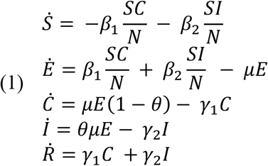 where S is the population of susceptible individuals and E are exposed individuals incubating the disease, and who eventually become infected. After the incubation period, 1/μ, we assume individuals will either be asymptomatic or mildly infected and will not be detected, C, or will have moderate to severe symptoms, I, which would result in detection. The parameter θ, describes this unknown value. Finally, we assume that individuals will either recover, die, or remove themselves from transmission through self-quarantine until they recover at rate γ.
Bayesian estimation of model parameters
Our goal was to estimate the ranges of parameters that would fit the data of the beginning of an outbreak in a country, assuming that initially the effects of distancing and other measures to control the disease are largely absent and thus the data are largely representative of the transmission dynamics but that some proportion of the infected population is not observed. Data on outbreaks in Italy, Spain, and South Korea were obtained from the Center for Systems Science and Engineering at Johns Hopkins University [1] (Figure 1). We fit the model to the observed data assuming that the first observed case was in the more severe group. We constrained our fit to the early part of the outbreak in each country, before widespread quarantines or extensive testing altered the path of the disease. For Italy this was from January 22, 2020 to March 20, 2020, for Spain this was from January 22, 2020 to March 30, 2020, and for South Korea this was from January 22, 2020 to March 5, 2020. To estimate the credibility of parameters, we used Monte Carlo (MC) to sample the parameter space with a uniform prior density with bounds and used acceptance and rejection sampling to approximate a posterior distribution of the parameters. The error between the results of the model yielding the expected number of observed cases and the observed number of cases is considered to be normally distributed with Norm (0, σ). The variance (σ2) is estimated as the difference between the model with the optimal parameter set and the observed number of cases. Reported parameter estimates are the medians of the posterior distributions, and 95% credible intervals from quantiles of the posterior distribution. The goal of the Bayesian parameter estimation is to approximate a posterior probability density function of the parameter. MC sampling of the parameter space was based on the number of reported active cases, recoveries and deaths. Specifically, we fit projected cases in the I compartment to active cases (confirmed cases minus recovered cases and deaths) and the R compartment to the sum of recovered and deaths. While traditional unbiased curve-fitting methods yield a set of parameter estimations that capture observed data, they do not account for known prior belief on parameter ranges. A Bayesian approach to parameter estimation allows us to quantify the credibility of one set of model parameters. This approach is extremely powerful as it provides a range of credible parameters in which the model can fit the observed data. Parameter bounds were based on disease dynamics literature and expert judgement (Table 1).
Parameters estimation from other literature
To assess the biological relevance of the parameters, we calculated the R0 of model, based on the dominant eigenvalue of the next generation matrix. The infection subsystem of the model can be described by equations (2).

We use a linearization of the infection subsystem, similar to the formulation outlined by Diekmann et al. [24],
 where the matrix T represents the transmission matrix that captures the number of transmissions from the susceptible compartments. The matrix M represents the transition between compartments within the infection subsystem. Specifically, T is equal to
 and M is equal to

From this formulation, we can mathematically construct the next generation matrix W, which is defined as
 which would equate to
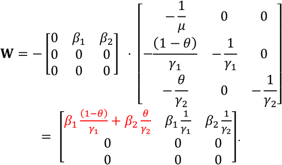
R0 is equal to the dominant eigenvalue of W (highlighted in red), which is equal to

Biological Parameters
To assess fit, determine model parameter priors for the model fits, and provide context for the analysis, we conducted a search of all literature already published on the biology and transmission of COVID-19. The majority of this literature was on pre-print servers such as medRxiv, bioRxiv and SSRN’s First Look (Table 1), and most data estimates were reliant upon small studies with wide variability. From this literature, we found an estimate for the incubation period, defined as the time from exposure to onset of illness, of 4.8±2.6 days [25]. The proportion of the population with no/mild/moderate symptoms was estimated to be as high as 85% of the population [26]. The infectiousness period, γ, was estimated to be 4.9 days (95% CrI: 3.3 – 5.9) based on the dynamics of earlier coronaviruses, though symptomatic and hospitalized cases likely have a longer recovery time than mild/asymptomatic cases [27]. Finally, we estimated the transmission rates, β1 and β2, based on calculations of the basic reproduction number, R0, of COVID-19 and clearance estimates. Values for R0in the literature range from 1.4 to 7.1 [11,28–30]; given these values we assumed that the transmission rate for β was likely between 0.1 and 0.9.
We first fit the data assuming only that transmission from our unobserved group (β1) was lower than from the symptomatic observed group (β2), as mild/asymptomatic cases are likely to shed fewer viruses and thus be less transmissible. Thus, we constrained β1 and β2 to be between 0.1-0.5 and 0.5-0.9, respectively. We then refit the data by constraining our symptomatic fraction, θ, to be 50% or less. The main results are presented as the fitted values and the relative relationship to the known biology. As the process is stochastic, we were interested in the local maxima obtained from this procedure to guide understanding of the parameters and to assess the ability of the model to fit actual data with biologically plausible values.
Results
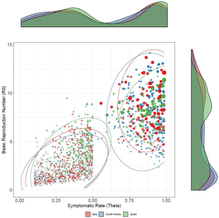
Assuming a uniform prior with no constraint on the fraction of the population that was symptomatic, θ, the parameter estimation from our MC sampling resulted in a posterior mean for the symptomatic rate of 0.89 (95% Credible Interval [CrI], 0.88-0.9), 0.91 (95% CrI, 0.9-0.92), 0.87 (95% CrI, 0.86-0.88) for Italy, Spain, and South Korea, respectively. The mean values of these parameter ranges resulted in a calculated R0 of 9.22 (95% CrI, 9.01-9.43), 9.14 (95% CrI, 8.99-9.29), and 8.06 (95% CrI, 7.82-8.3) for Italy, Spain, and South Korea, respectively, and generally followed a negative correlation with θ in our Bayesian estimation (Figure 2). Constraining the uniform priors of θ to only sample from 0.01 - 0.50, meaning the parameter estimation for asymptomatic rate could not be higher than 50 percent, results in R0 values of 2.56 (95% CrI, 2.41-2.71), 3.23 (95% CrI, 3.06-3.4), and 2.36 (95% CrI, 2.22-2.5) for Italy, Spain, and South Korea, respectively. These results were positively correlated with R0 such that higher fractions of symptomatic individuals resulted in higher R0 values. The resulting values for the parameter estimates are shown in Table 2.
MC Priors and Parameter Estimation Fits of Model for Italy, Spain and South Korea
Using Monte Carlo (MC) methods, we were able to generate 400 parameter samples from a prior distribution with acceptance-rejection sampling. In the figure, each set of sampled parameters of three countries, Italy, South Korea, and Spain, were generated which allow us to calculate the R0, basic reproduction number, and display those values against the symptomatic rate (θ). The probability distribution for R0and θ are displayed on the right and top, respectively. The size each point represents the relative inverse sum of square errors for each country, with larger sized points being a better fit. The ellipses encircle 95% of simulation runs for each scenario. The triangular points represent priors for θ that were bounded (constrained) between 0.01-0.5, while the circular points represent priors (unconstrained) that were bounded between 0.01 – 0.99.
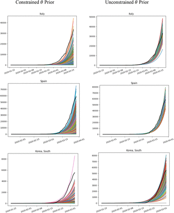
The overall fit of the model to the data was generally better in the unconstrained case, in which only a small fraction of the population is missed due to unobserved asymptomatic/mild infection (Figure 3). Variation between the two estimated scenarios was primarily governed by differences in the length of the infectiousness of the symptomatic group. In the high symptomatic case, the fit of the parameter produced mean infectiousness periods of 12-17 days, while in the constrained case the infectiousness period was estimated to be about 7 days.
Based on the 200 sets of parameters that were obtained from MC sampling, the severe infection outcomes are of each run for Italy are displayed in color, while the observed active cases are displayed in black. The left side show the MC sampling for priors for θ (symptomatic rate) that were bounded uniformly between 0.01-0.5 (constrained), while the right side represent priors that were bounded between 0.01 – 0.99 (unconstrained). Although, unconstrained parameters have a better fit to observed data, the constrained priors may capture the true dynamics of cases which will result in a relatively steeper increase.
Discussion
As COVID-19 spreads through the United States, questions remain as to the rate of disease spread, the extent of people infected, and the implications for policies regarding quarantines. We conducted this analysis to contribute to available disease models, which play an integral role in defining the policy choices of government officials. Accurate evidence that conforms to observed data is needed to aid those decisions. Our results suggest that there appear to be two dichotomies. The first assumes that most cases are discovered and the R0 of the disease is more than 8. The second assumes a lower R0, but a large fraction of the population is asymptomatically infected and excluded from official estimates of the disease spread. Given these scenarios, we believe the more likely case is that a large fraction of the population is asymptomatically infected, and the only question is what percentage.
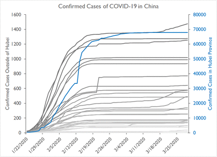
If the proportion of individuals that are asymptomatically infected is actually higher than initially assumed, waiting for the emergence of observed cases to impose travel restrictions is not a productive policy, because (i) there are likely far more infected individuals than are observed, and (ii) due to the long dynamics of the incubation period, there is a large proportion of people who are already infected but not yet infectious. Evidence from China suggests that the observed data trail reported infections by about two weeks. In other words, despite dropping transmission dramatically between January 15 and January 25, the rate of newly confirmed cases did not begin to level off both country-wide and within each local city until two weeks later (Figure 4).
The confirmed cases by localities outside of Hubei, China are shown for January 22nd, 2020 to March 30th, 2020. We can see similar exponential increases in cases were observed after the population is rescaled with respect to population inside Hubei Province.
Assuming a large fraction of the population is asymptomatically infected has important implications for policy because of herd immunity. While there have been some potential second cases, the vast majority of the evidence suggests that infected individuals develop immunity to circulating strains. As more of the population gains immunity, disease spread will slow. When transmissibility between contacts falls because of widespread immunity, the effective reproductive number is reduced, the disease spreads more slowly, and the threat posed by widespread numbers of infected individuals fades away. Such widespread immunity would allow restrictions to be lifted sooner, as most individuals would not pose a transmission risk to the general public and would abrogate the possibility of a second peak in the future. Understanding the potential risks requires serological surveys to be conducted as soon as possible in areas with high and low numbers of cases to understand how much the disease has been spreading and to inform better policies regarding quarantines.
Finally, the troubling implication of these results is that asymptomatic rates are estimated to be ∼50%. Based on the fits from the model, this would suggest that the R0 of COVID-19 may be higher than 2.5. A high R0 combined with large numbers of asymptomatic and mildly infected individuals could account for the “bomb-like” dynamics of COVID-19. In New York City, the rate of confirmed cases has been doubling roughly every 2 days. This is faster even than Italy where the rate of doubling was approximately every three days. Recent data on mortality in the NYC region suggests that this rapid increase in cases is not just the effect of rapid increased testing, as the number of deaths is growing at a similar rate as the case load with an approximate two-week lag (Figure 5). This mortality rate is, at least for the moment, substantially higher than the rate in Italy (Figure 6). This suggests that densely populated urban areas may facilitate more rapid spread of the disease and have even higher reproductive numbers. Given the strong connectivity between China and NYC, it is likely the first cases of COVID-19 arrived in NYC by late January, yet the first case was not observed until late February and there was no “explosion” until mid-March. This should be a cautionary tale to other cities that are not as connected to international travel as NYC or are in the Southern Hemisphere, where potential seasonal differences may have led to lower transmission rates in February and March [31]. Postponing policy action until the outbreak is well underway, as NYC and Italy did, is thus much less effective in containing the virus. Only by extensive and early restrictions can the bomb-like dynamics of the disease be averted. In South Korea, the dynamics initially appear similar, but the introduction of widespread testing likely led to the discovery of much larger numbers of less severe cases, which bent the curve. However, as the case of Hong Kong demonstrates, relaxing these policies before the disease has spread widely enough to provide herd immunity leads to rapid growth in cases within a couple of weeks [32]. Without a vaccine, cities and countries will need to manage the spread of the virus so that the number of hospitalized individuals will not exceed capacity. This is a difficult option but the only rational policy until more progress is made in vaccine development or therapeutics.
Confirmed cases and deaths in NYC. There appears to be a consistent lag, but similar rate of increase in deaths compared to cases, suggesting that the increase in confirmed cases is not due primarily to testing changes, but to actual disease dynamics.
Per capita death rate in NYC compared to Italy.
Conclusion
The explosive nature of COVID-19 disease dynamics is likely the result of large fractions of asymptomatic and mild cases leading to rapid and silent spread throughout the community. However, even this cannot explain the dynamics of disease spread alone in certain areas, such as NYC, without assuming that the reproductive number, or R0, is higher than the reported values based on severe symptomatic cases.
Data Availability
Data derived from public domain resources
Funding
This work was funded by the Centers for Disease Control and Prevention (CDC) MInD-Healthcare Program (Grant Number 1U01CK000536). SL was supported by The National Science Foundation (CCF 1917819). DM was also supported by the Agency for Healthcare Research and Quality (AHRQ) Patient Safety Learning Laboratory program.


