
ABSTRACT
Background The relationship between skin diseases and mental illnesses has been extensively studied using cross-sectional epidemiological data. Typically, such data can only measure association (rather than causation) and include only a subset of the diseases we may be interested in.
Objective In this paper, we complement the evidence from such analyses by learning an overarching causal network model over 12 health conditions from a Google search trends public data set.
Methods We learned the network model using a dynamic Bayesian network, which can represent both cyclic and acyclic causal relationships, is easy to interpret and accounts for the spatio-temporal trends in the data in a probabilistically rigorous way.
Results The average R2 for a condition given the values of all conditions in the previous week is 0.67: in particular, 0.42 for acne, 0.85 for asthma, 0.58 for ADHD, 0.87 for burn, 0.76 for erectile dysfunction, 0.88 for scars, 0.57 for alcohol disorders, 0.57 for anxiety, 0.53 for depression, 0.74 for dermatitis, 0.60 for sleep disorders and 0.66 for obesity. Results confirm the large number of cyclic relationships between the selected health conditions and the interplay between skin and mental diseases. For acne, we observed a cyclic relationship with anxiety and attention deficit hyperactivity disorder (ADHD) and an indirect relationship with depression through sleep disorders. For dermatitis, we observed directed links to anxiety, depression and sleep disorders and a cyclic relationship with ADHD. We also observe a link between dermatitis and ADHD and a cyclic relationship between acne and ADHD. Furthermore, the network includes several direct connections between sleep disorders and other health conditions, highlighting the impact of the former on the overall health and well-being of the patient.
Conclusions Mapping disease interplay, indirect relationships and the key role of mediators, such as sleep disorders, will allow healthcare professionals to address disease management holistically and more effectively. Even if we consider all skin and mental diseases jointly, each disease subnetwork is unique, allowing for more targeted interventions.
Introduction
Skin diseases and mental illnesses have been extensively studied. However, they are commonly investigated in isolation: the interplay between different skin diseases, between mental illnesses, and between skin diseases and mental illnesses are ignored, limiting our understanding of their aetiology. Skin and brain may interact in four ways: skin-to-skin, brain-to-brain, skin-to-brain and brain-to-skin. Skin-to-skin interactions, or skin disease associations, may arise because of the general altered skin barrier function shared by all inflammatory skin diseases1; because of the use of topical drugs that induce an alteration of the skin barrier function or other skin reactions2,3; and because of common aggravating mental and environmental risk factors4,5.
As for brain-to-brain interactions, there is a growing consensus among psychiatrists that the boundaries between mental disorders, which often overlap in signs and symptoms, are not clear: a recent study shows that mental diseases share a large number of genetic variants6. Anxiety and depression, for example, have a genetic correlation of 0.79, while ADHD has a correlation of 0.39 with anxiety and 0.52 with depression. More developments are needed to take into account these overlapping genetic contributions to reduce diagnostic and treatment heterogeneity of psychiatric disorders.
Skin-to-brain interactions have largely been investigated through the evaluation of the impact of skin diseases on mental health, mainly anxiety, depression and attention deficit hyperactivity disorder7–13. This relationship has also been studied indirectly through the impact of skin diseases on symptoms directly related to mental illnesses such as depressive symptoms, social isolation and loneliness14–16. A second important pathway is through mediators like the quality of sleep in connection with pruritus17–20. Over-representation of sleep disorders has been observed in patients with psoriasis, atopic dermatitis, hidradenitis suppurativa and vitiligo21–24. More recent works study the reverse effect of sleep deprivation on skin disease through the bi-directional relationship between sleep and the immune system25. This link is thought to contribute to the chronic inflammation observed in many skin diseases. Therefore, dermatologists should emphasise sleep hygiene in their practice.
Dermatologists studying brain-to-skin interactions have been arguing that stress, anxiety and depression can aggravate or precipitate the onset of most inflammatory skin diseases. The COVID-19 pandemic provided strong evidence supporting this hypothesis, with dermatologists reporting an increase in the incidence of flares during this period26. Unfortunately, this effect is difficult to quantify because patient access to medical treatment was restricted during lockdown periods when stress, anxiety and depression were most likely to develop. The hypothalamic pituitary adrenal (HPA) axis is responsible for responding to psychological stress, which produces both pro- and anti-inflammatory effects on the skin4 in turn. Initially, the release of pro-inflammatory cytokines by the corticotropin-releasing hormone (CRH) starts a quick inflammatory process. However, CRH also triggers a slower anti-inflammatory process that leads to the release of glucocorticoids (cortisone, cortisol). Studies have shown that pro-inflammatory cytokines induce mast cell activation, promoting immune dysregulation and neurogenic inflammation27,28. They are known to play a role in allergic reactions as well29. Inflammatory skin diseases share a common link with the quality of the skin barrier function: the enzyme 11β -hydroxysteroid dehydrogenase type I, which is responsible for the transformation of cortisone (inactive form) into cortisol (active form), is a marker of barrier function impairment30. Anti-psychological stress interventions like SSRI reduce both enzyme concentration and improved barrier function.
Psychological stress is not only an aggravating factor for skin diseases but may also trigger diseases like vitiligo31, psoriasis32, seborrheic dermatitis33, trichotillomania, excoriation disorder and delusions of parasitosis34 in individuals with genetic susceptibility.
Complementing this epidemiological evidence with a model of the interplay between these four classes of interactions is crucial to improving the diagnosis and treatment of skin diseases and mental illnesses in medical practices. Modelling this interplay using epidemiological data is very difficult because of the lack of comorbidity studies with a longitudinal design. In this paper, we consider the search trends infodemiologic data available in the Google COVID-19 Public Data, an analysis-ready large longitudinal data set35. It is not the first time that this data set has been used to complement epidemiological insights for achieving a larger sample size or for disease early detection36. The intuition behind its use is that many patients perform online searches about their putative conditions before visiting a physician36,37. We can then assume a non-negligible association between the frequency of online searches for specific diseases and the actual incidence of those diseases in physicians’ diagnoses. Restricting ourselves to searches performed on Google is not a significant limitation because of the prevalence of its use: 8.5 billion queries are processed by Google every single day38. At the time of this writing, a search of PubMed titles and abstracts with the keywords “search trend” and “Google search” yielded 1489 results in 2020, 59% more than in 2019. This volume has been maintained in 2021 and 2022. The COVID-19 pandemic has highlighted how such data can be used to track pandemics and, more interestingly, to study longitudinal patterns of disease progression in several healthcare domains39,40. However, poor documentation practices and high heterogeneity in methods have led to conflicting findings41. Previous infodemiologic studies based on Google search trends relied on keyword matching, which is likely to miss many classes of queries, and many of them did not incorporate query translation, which may result in significant loss of information in countries like the US where multiple languages are in common use42. To overcome these two issues, Google leveraged the latest advancements in natural language processing (NLP) for query classification and translation, including state-of-the-art transformers built using massive corpus with deep neural networks43, to create the COVID-19 Public Data set. Training on large corpora makes them more accurate in classifying diseases even with little to no fine-tuning (respectively, zero-shot classification without additional supervised learning44 and with few-shot classification with a small number of examples45).
We will use the Google COVID-19 Public Data set to model the interplay between skin diseases and mental illnesses using dynamic Bayesian networks (dynamic BNs)46. This class of graphical models has a unique set of advantages: they provide a graphical representation of the interactions between diseases; they can be learned automatically from data, from expert knowledge, or a combination of both; and they can be used as diagnostic or prognostic support systems because they can easily evaluate any scenario of interest. Most importantly, unlike the more common correlation networks, dynamic BNs represent interactions as directed arcs that can disambiguate causes and effects47,48. This ability is crucial in finding appropriate targets for treatment, thus avoiding symptomatic treatment and improving clinical outcomes, and in differentiating unidirectional cause-effect relationships from feedback loops. As a result, dynamic BNs provide a clearer picture of the interplay between the skin and the brain and, at the same time, they are better suited to design treatment regimes.
Results
The data set used in this work is publicly available at the URL listed in the Data Availability. We considered the web search queries collected weekly from users in the United States between 2020-03-02 and 2022-01-24 (100 weeks). We focus on the following 12 conditions (with abbreviations): obesity (“OBE”), acne (“ACNE”), alcoholism (“ALC”), anxiety (“ANX”), asthma (“ASTH”), attention deficit hyperactivity disorder (“ADHD”), burn (“BURN”), depression (“DEP”), dermatitis (“DER”), erectile dysfunction (“ED”), sleep disorder (“SLD”) and scar (“SCAR”). We detail the mapping between these conditions and the variables in the search trends in Supplementary Table 1. To avoid a very sparse data set, we remove symptoms with more than 30% missing data. The focus is on skin diseases, excluding very general symptoms like “Lesions”, “Skin conditions”, “Infection”, “Inflammation” and “Skin ulcer” or with potential confusion like “Xeroderma”. The second set of symptoms are mental conditions with a focus on anxiety, depression and ADHD, the most studied mental disease in dermatology. We retain asthma for its documented link with atopic dermatitis and anxiety49,50. Obesity is a comorbidity that plays an important role in mental disorders like anxiety51, so its presence is justified to control confounding in some relationships. Obesity may also trigger some skin diseases like atopic dermatitis and psoriasis52,53. Erectile dysfunction is selected because it is considered a probable consequence of mental disorders and sleep deprivation54,55. Considering additional health conditions might allow the network to recover more information but is likely to produce dense networks that are difficult to interpret and make computations cumbersome. For each of these conditions, we retrieved from the Google COVID-19 Public Data set the relative frequency in web search queries of the relevant search terms in each county of each US state over the period. Therefore, the resulting data set we used for the analysis is a weekly multivariate time series over 12 health conditions for each county and state with the relative frequencies of the web search queries normalised at the county level. Missing data were imputed, and we confirmed the accuracy of the imputation process to be satisfactory. (See the Methods for details). The overall number of observations for each condition given by 2879 counties over 50 states and 100 weeks is 287900.
The dynamic BN model we learned from these data to investigate the skin-brain-skin connections among the conditions above is shown in Figure 1. The model should be read as follows: each node corresponds to one of the conditions above, and arcs represent direct probabilistic associations. Nodes not connected by an arc are indirectly associated if we can find a path that connects them without passing through any node corresponding to conditions we may be controlling for, or conditionally independent otherwise.

The dynamic Bayesian network linking skin and brain conditions learned from the Google COVID-19 Public Data Set.
The interactions between these conditions, which can be unidirectional effects and feedback loops, were learned in an unsupervised manner to validate known relationships from the literature and discover new putative ones. To reduce false positives (which implies including spurious arcs in the dynamic BN in this context), we structured the dynamic BN to account for the temporal and spatial dependence structure of the data, and we integrated model averaging via bootstrap resampling in the learning process. Furthermore, we tuned the learning process by penalising the inclusion of arcs in the dynamic BN to find the optimal balance between predictive accuracy and the need for a sparse network. The large sample size of the Google COVID-19 Public Data Set gives us enough statistical power to detect even marginal effects. However, an overly dense network model would hardly be interpretable from either a qualitative or quantitative point of view: it would be difficult to examine visually, and it would fail to formally identify which pairs of conditions are independent or conditionally independent. Therefore, we chose the final dynamic BN shown in Figure 1 to have about three arcs for each condition. Even so, the average predictive accuracy across all conditions is 99.96% of that of the dynamic Bayesian network learned in the same way but with no penalisation. In absolute terms, the R2 for each condition given the values of all conditions in the previous week are 0.42 for ACNE, 0.85 for ASTH, 0.58 for ADHD, 0.87 for BURN, 0.76 for ED 0.88 for SCAR, 0.57 for ALC, 0.57 for ANX, 0.53 for DEP, 0.74 for DER, 0.60 for SLD and 0.66 for OBE (average 0.67). The strength of the arcs, our confidence that they are statistically significant, are reported in Supplementary Table 2. As expected, most are identical or close to 1 (where 0 represents a complete lack of confidence and 1 is the strongest possible confidence). Note that the model allows us to give a causal interpretation to the arcs within the frameworks of Granger’s and Pearl’s causality. (See the Methods for more details.) We show in Figure 2 how the variability in ACNE, ANX, DER, DEP, SLD and ADHD is explained by the respective parents: these traits are of particular interest to us. In particular, we note that ASTH explains a nontrivial proportion (0.235) of the variability of ACNE in the following week, less than OBE (0.264) but more than ANX (0.216). However, the association between the ASTH and ACNE is not well established in the literature. We attribute this finding to the fact that ANX is connected to all of ASTH, ACNE and OBE, which may allow for confounding in models that do not consider them simultaneously. For instance, such confounding may arise because of the feedback loop between ACNE and OBE (which are both connected to ANX) unless OBE is controlled for. Our model supports the hypothesis that ASTH and ACNE are only weakly linked (in the same week) after controlling for ANX (in the previous week): if we perform inference on the dynamic BN as described in the Methods, the proportion of the overall variance of ACNE explained by ASTH is only 0.0041. Stratifying by ANX (low: bottom quartile of search query frequencies; high: top quartile; average: second and third quartiles) reveals that the proportion of explained variance is even smaller when ANX is average or low (0.0046, 0.0036, respectively) compared to when ANX is high (0.0053). Furthermore, the model supports the hypothesis that the feedback loop between ACNE and OBE is driven by ANX: ACNE explains OBE (proportion of variance: 0.622) and OBE explains ACNE (proportion of variance: 0.264). However, after controlling and stratifying for ANX using BN inference, OBE only explains proportions 0.016 (high ANX), 0.017 (low ANX) and 0.013 (average ANX) of the overall variability of ACNE in the same week. The same is true for ACNE, which explains similar proportions of the variance of OBE.
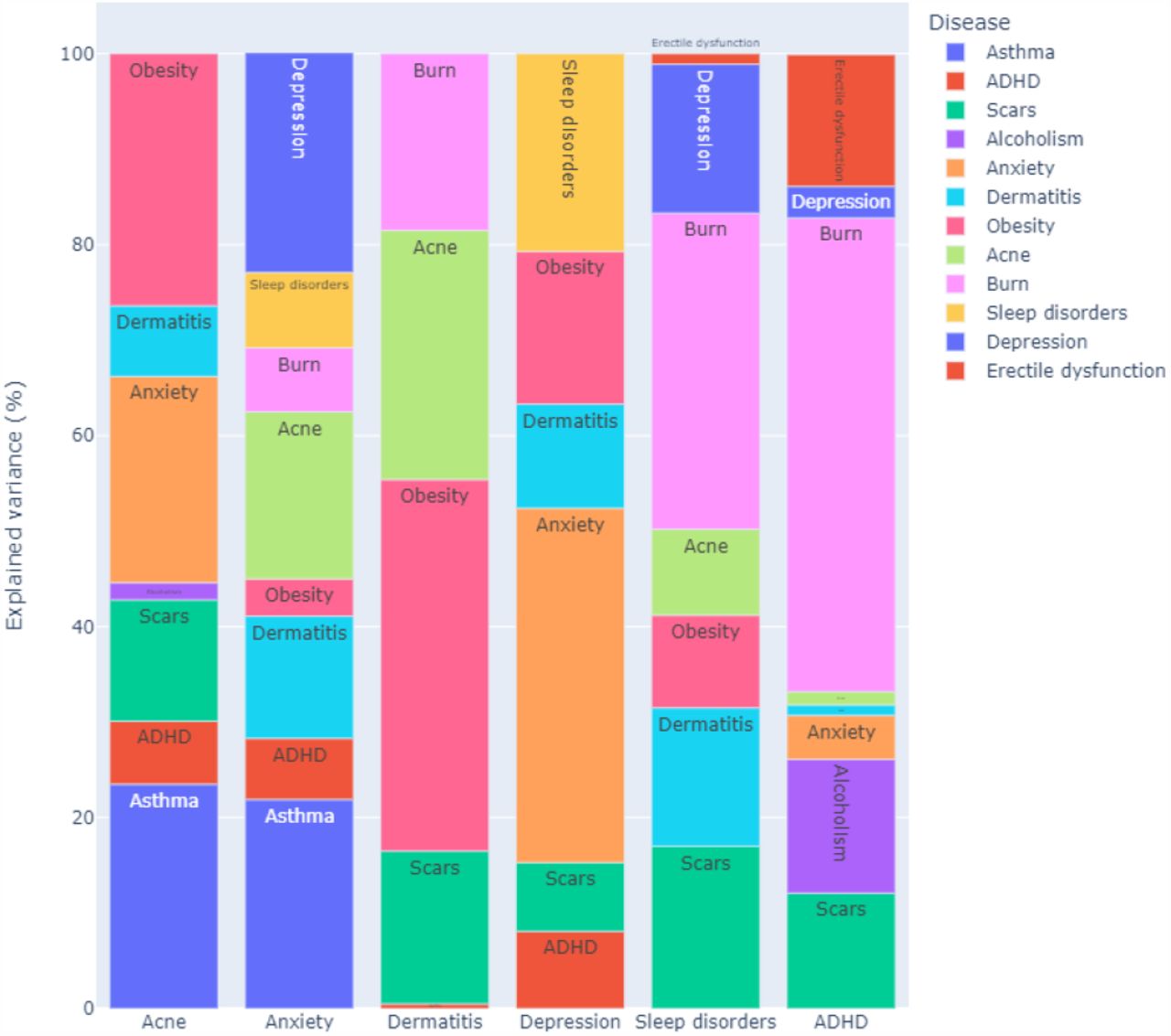
Proportions of the variance of some conditions of interest explained by their parents in the network shown in Figure 1. The conditions are acne (ACNE), anxiety (ANX), depression (DEP), dermatitis (DER), sleep disorder (SLD) and ADHD. The proportions are computed excluding the contribution of the condition itself from the previous time point in the data.
These results confirm the cyclic relationships between skin and mental health conditions. Figure 2 highlights the importance of each trigger for the six health conditions. Depression is mainly driven by mental disorders and sleep disorders but dermatitis explains a significant proportion of its search popularity. Anxiety triggers are more diverse: skin conditions like acne and dermatitis play an important role. Triggers of ADHD, learned in an unsupervised way by the dynamic BN, give a new insight into the disease. It is already known that ADHD is associated with a risk increase of burn injuries and scarring (from burns): these data suggest that an increase in burn injuries may lead to ADHD diagnosis.
For acne, we observed a strong, direct cyclic relationship with anxiety and ADHD and an indirect relationship with depression through sleep disorders. For dermatitis, we observed directed links to anxiety, depression and sleep disorders and a cyclic relationship with ADHD. We also observed a link between dermatitis and ADHD, and a cyclic relationship between acne and ADHD. The role of mediators like sleep disorders is confirmed in the network with a significant impact on anxiety and depression. Acne, burns, scars and dermatitis directly impact sleep disorders. The learned BN visualises multiple disease relationships in a single picture.
Discussion
Even though the modelled causations are infodemiologic and not clinical, the results confirm the interplay between skin diseases and mental illnesses. Several skin-to-skin, brain-to-brain, skin-to-brain and brain-to-skin relationships are highlighted in the model. It is interesting to see well-known clinical relationships reproduced in the dynamic BN and put into a larger context with deeper explanations.
The large number of feedback loops supports the existence of vicious circles in which diseases exacerbate each other until treated appropriately. The results cannot elucidate the starting point of these circles but emphasise the need for more holistic disease management for dermatologists and psychiatrists. Dermatologists should take into account the mental health of their patients, and psychiatrists should take into account the skin problems of their patients.
The results also highlight the essential role of key mediators, like sleep disorders, that establish a bridge between the skin and the brain. We should not ignore these disorders if we want to act effectively on skin and mental health. Furthermore, not controlling for comorbidities like obesity may lead to spurious conclusions, hiding the existing relationships.
Even if we consider all skin and mental diseases jointly, each disease subnetwork is unique, allowing for more targeted interventions. The conditional independence property of BNs allows for this kind of focus without loss of information.
In this work, we also wanted to raise awareness of the importance of measuring causality with appropriate study designs and statistical methods leveraging multiple conditions in longitudinal monitoring and allowing feedback loops to reproduce the natural cycle of human health. This may significantly reduce the number of measured associations and highlight a focused set of preferential targets for intervention.
The second important objective of this study was to provide guidelines for better use of search trends data to ensure robust findings. Firstly, query classification using a keywords approach may fail to capture relevant information, leading to low reproducibility across researchers. Using the latest AI breakthroughs in natural language processing for query translation and classification will ensure better reproducibility of studies.
Secondly, choosing models that can capture the main features of search trends data is necessary to avoid several sources of bias. We provided a detailed methodology to deal with missing data, space and time dependencies, the lack of sparsity in the network due to the size of the data set, model interpretability and other considerations.
The marked discrepancies between the conclusions of studies dealing with this type of data can be attributed to how queries were classified and processed. Standardising these two tasks will demonstrate the high potential of these data to complement clinical evidence for a more positive impact on public health.
Media coverage, a common source of bias in internet data, should also be taken into account and may be mitigated with big data sets.
Methods
All analyses were performed using R56 and the packages nlme57, lme458, imputeTS59 and bnlearn60.
Missing data management
The Google COVID-19 Public Data Set originally contained missing data, either single data points or whole time series for specific counties and periods. The proportion of missing data in individual conditions ranged from 0% to 16%. We explored different methods to impute them for both individual time series (exponentially weighted moving average, interpolation) and multivariate time series (Kalman filters) using the imputeTS R package. To assess their performance, we used the complete observations and artificially introduced 2%, 5%, 10% and 20% missing values individually and in batches of four to simulate both random missingness and lack of measurements over one month. All combinations of missing data patterns, proportions, and algorithms produced average relative imputation errors between 10% and 14%, suggesting that all imputation methods perform similarly (Supplementary Figures 1 and 2). Finally, we chose an exponentially weighted moving average imputation because of its simplicity. Imputing some combinations of conditions and counties was impossible because of the insufficient number of observed values; we dropped them from the data, reducing the overall sample size to 287866.
Spatio-Temporal dependence structure of the data
The Google COVID-19 Public Data Set was collected over time and in different US states and counties and, therefore, presents marked spatio-temporal patterns of dependence between observations. We will summarise them here because they are crucial in our modelling choices.
To be consistent with the assumptions of the dynamic Bayesian network we will describe below, we quantify the magnitude of spatial and temporal dependencies with the proportion of the variance of the conditions that they explain as random effects in a mixed-effect model [58]. For spatial dependencies, we further distinguish between the variance explained by the state and by the county. For time, we assume an autocorrelation of order 1 (that is, each condition is correlated with itself at the previous time point). The proportions for each condition and the average over all conditions are shown in Supplementary Figure 3. On average, states explain 12% of the variance of the conditions (min: 7%, max: 16%), counties explain 49% (min: 23%, max: 84%), and counties together with autocorrelation explain 64% (min: 35%, max: 86%).
Dynamic Bayesian networks
Bayesian networks (BNs)46 are a graphical modelling technique that can leverage data combined with an expert’s prior knowledge to learn multivariate pathway models. The graphical part of the BN is a directed acyclic graph (DAG) in which each node corresponds to a variable of interest (here one of the conditions) and in which arcs (or the lack thereof) elucidate the conditional dependence (independence) relationships between the variables. The implication is that each variable depends in probability on the variables that are its parents in the DAG: as a result, the joint multivariate distribution of the data factorises into a set of univariate distributions associated with the individual variables. This property allows automatic and computationally efficient inference and learning of BNs from data and has made them popular for analysing clinical data61–63. In particular, BN inference can automatically validate arbitrary hypotheses: in the simplest instance, a BN is used as a generative model and hypotheses are validated by stochastic simulation.
To account for the spatio-temporal nature of the data, we use a particular form of BN called a dynamic BN in which each variable appears in the DAG as a separate node at each time point. The key advantage of dynamic BNs is that, unlike classical BNs, they can represent feedback loops by allowing each variable in a pair to depend on the other across time points: for instance,  and
and  implies a feedback loop between X1 and X2 across two consecutive time points t0 and t1. Arcs are only allowed to point forward in time from a variable measured at t0 and one measured at t1 to ensure that they are semantically meaningful and to be able to relate the dynamic BN to the Granger causality47 and Pearl Causality frameworks48. We disallow “instantaneous arcs” between variables measured in the same time point for similar reasons. With these restrictions, we can construct a cyclic directed graph that can represent feedback loops from the DAG by folding the nodes corresponding to the same variable at different time points into a single node. As a result, pairs of arcs like
  and
and  are transformed into cycles of the form X1 ⇆ X2; and arcs like
  become loops that express autocorrelation.
As for the distributions of the variables, we assume that 1) the search query frequencies in any given week can depend in probability on those in the previous week but not on older ones, and 2) the data are stationary, so we only need to model the dependence between two generic consecutive times t0 and t1. These assumptions allow us to parameterise the dynamic BN similarly to a vector auto-regressive time series64: each condition Xi in each county is therefore modelled using a linear regression model of the form
 at time t1 and
 at time t0. Here pa(·) denotes the parents of the variable, μi is the intercept, the βi are the associated regression coefficients, and the εi are normally distributed residuals with mean zero and some variance specific to each node. The contribution of each parent to the linear regression can thus be naturally measured by the associated explained variance in the model (ANOVA). Conditions have different scales arising from the different popularities of the corresponding search queries: to make them easier to compare in the Results, we normalise the variance explained by each parent into a proportion (that is, we divide it by the total explained variance of all parents). In doing so, we omit the contribution of the condition itself: in the auto-regressive model we are considering, auto-correlations are strong enough to make the contributions of other conditions appear less significant for purely numerical reasons.
In addition to accounting for the time dimension, the dynamic BN incorporates the spatial structure of the data. Assume that each condition has a different baseline value in each county that does not change over time. Then the local distribution of each condition at time t1 is regressed against itself at time t0 (same county, previous time point). The different baseline for the state then appears on both sides of the equation and can be accounted for in the regression model.
We learned the dynamic BN from the data by choosing the optimal DAG that maximises the penalised log-likelihood
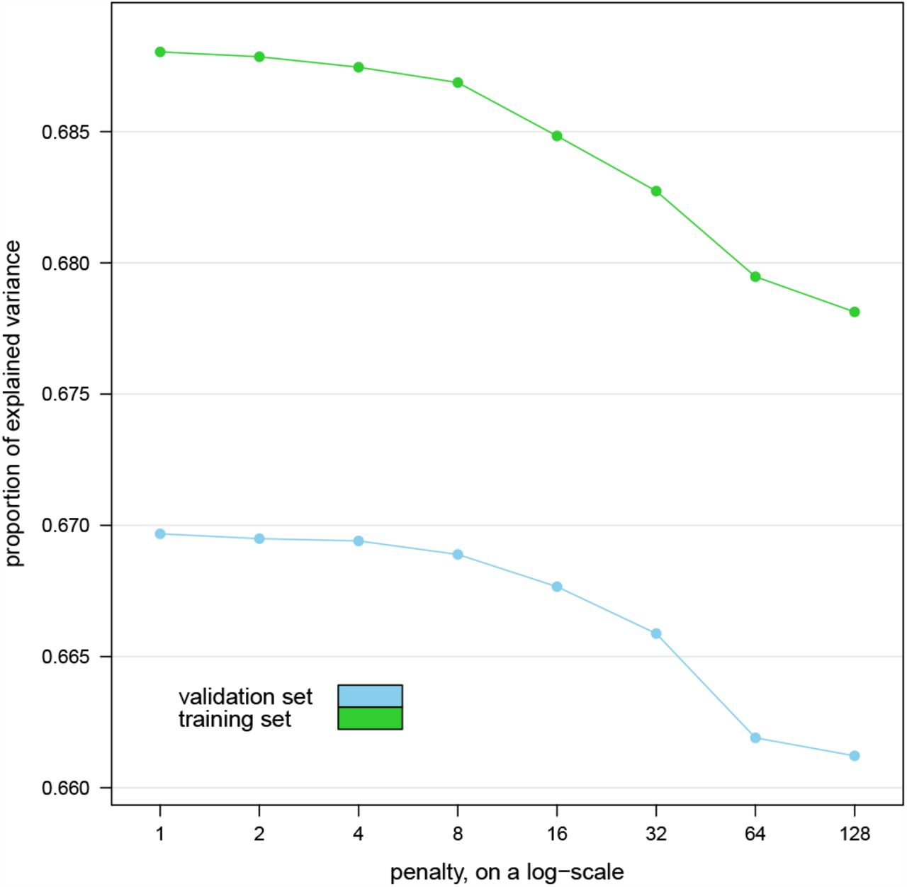
 where p is the number of parameters of the dynamic BN and n is the number of observations in the data, using the hill-climbing greedy search algorithm65. We then estimated the parameters of the dynamic BN (the intercepts μi and the regression coefficients βi) with the chosen DAG using maximum likelihood. To ensure that the DAG is as sparse as possible without sacrificing predictive accuracy, we chose the penalty coefficient w by learning the dynamic BN with w = 1, 2, 4, 8, 16, 32, 64, 128 on the first 52 weeks of data and then computing the average proportion of variance explained over all conditions in the remaining weeks of data acting as a validation set. For reference, w = 1 gives the Bayesian Information Criterion (BIC)66. Larger values of w penalise the inclusion of arcs in the DAG by increasingly large amounts, effectively decreasing the value of the penalized likelihood if the associated regression coefficients are small.
The resulting proportions of explained variance are plotted against w in Figure 3. We observe no marked decrease in predictive accuracy until w = 4, which we choose as the best trade-off with the sparsity of the DAG. For reference, the dynamic BN learned with w = 1 has 123 arcs while that learned with w = 4 has 87 arcs with a predictive accuracy that is 99.96% of the former model. We also note that the variance explained by the dynamic BNs in the validation set is not markedly different from that in the training set they were learned from, suggesting no overfitting.

Average proportion of explained variance over all conditions explained by the dynamic Bayesian networks learned from the first year’s worth of data (training set) in the remaining weeks (validation set) for various values of the penalty coefficient w.
The large number of observations available on each condition gives the dynamic BN enough statistical power to detect even marginal effects from the data and thus to include them as arcs in the model, resulting in an overly dense DAG. The fact that increasing w and dropping many of those arcs has a limited impact on predictive accuracy suggests that the relationships they express may be of limited clinical relevance for diagnostic or prognostic purposes.
Furthermore, we used model averaging to reduce the potential of including spurious arcs in the BN. We implemented it using bootstrap aggregation: we extracted 500 bootstrap samples from the data, learned the DAG of a dynamic BN from each of them, and then constructed a consensus DAG containing only those arcs that appear with frequency higher than the data-driven threshold67. Each frequency measures the strength of the corresponding arc, that is, of our confidence that the arc is supported by the data: a value of 0 represents a complete lack of confidence, whereas a value of 1 represents perfect confidence. To further prevent patterns in the data from impacting the consensus model, we increased the variability of the bootstrap samples by randomising the order of the variables and by reducing their size to 75% of that of the original data.
Finally, we assessed the impact of the spatio-temporal structure of the data on structure learning to motivate using dynamic BNs. For this purpose, we performed both structure and parameter learning as described above to fit a classical (that is, static) BN in which variables are not replicated across time points. As a means of comparison, we learned a second static BN from the data after removing their spatio-temporal structure with the mixed-effect model we used above to quantify the proportion of variance explained by the counties and the temporal autocorrelation. If we only perform parameter learning, we find that 63% of the regression coefficients are inflated by a factor of at least two compared to those we learn after removing the spatio-temporal structure from the data. The sign is different for 29% of them. If we perform structure learning from both sets of data, we find that 71% of the arcs differ between the two. The reason is that a classical, static BN is a misspecified model, and the dependence relationships between the variables are confounded with space-time dependencies between the data points. This supports our choice to use a dynamic BN instead.
Code availability
The code used for the analysis is publicly available at the URL: https://www.bnlearn.com/research/loreal21
Data availability
The Google COVID-19 Public Data Set is publicly available at the URL: https://console.cloud.google.com/marketplace/product/bigquery-public-datasets/covid19-public-data-program
Author contributions statement
M.S. analysed the data and wrote the software for the analysis. D.K. conceived the study and interpreted the clinical results. S.S. conceived the study, collected the data and interpreted the clinical results. All authors wrote and reviewed the manuscript.
Competing interests
The authors declare no competing financial or non-financial interests.
Supplementary information
Supplementary Table 1: Mapping between the variables in the Google COVID-19 Public Data Set and the conditions discussed in this paper. When multiple variables map to the same condition, the search query frequencies from those variables were aggregated to give a single overall frequency for the condition.
Supplementary Table 2: Arc strengths for the dynamic Bayesian network model shown in Figure 1. “From” denotes the node at the tail of the arc, “To” denotes the node at the head of the arc and “Arc strength” is the frequency of the arcs in the bootstrapped models.
Supplementary Figure 1: Average relative error (in absolute value) for the missing data imputation algorithms with individual missing values amounting to 2%, 5%, 10% and 20% of the total.
Supplementary Figure 2: Average relative error (in absolute value) for the missing data imputation algorithms with values missing in 1-month batches (4 consecutive weeks) amounting to 2%, 5%, 10% and 20% of the total.
Supplementary Figure 3: Proportion of the variance of each condition explained by the US states, by the counties and by the counties together with the temporal autocorrelation. The average for each of them over all conditions is reported at the bottom.
Acknowledgements
We thank Dr. Katrina Abuabara for her comments and suggestions on an early draft of this paper.
Footnotes
Minor edits upon resubmission to a new journal.
References


