
Abstract
Infant mortality remains high and uneven in much of sub-Saharan Africa. Given finite resources, reducing premature mortality requires effective tools to identifying left-behind populations at greatest risk. While countries routinely use income- or poverty-based thresholds to target policies, we examine whether models that consider other factors can substantially improve our ability to target policies to higher-risk births. Using machine learning methods, and 25 commonly available variables that can be observed prior to birth, we construct child-level risk scores for births in 22 sub-Saharan African countries. We find that targeting based on poverty, proxied by income, is only slightly better than random targeting, with the poorest 10 percent of the population experiencing approximately 10 percent of total infant mortality burden. By contrast the 10 percent of the population at highest risk according to our model accounts for 15-30% of infants deaths, depending on country. A hypothetical intervention that can be administered to 10% of the population and prevents just 5% of the deaths that would otherwise occur, for example, would save roughly 841,000 lives if targeted to the poorest decile, but over 1.6 million if targeted using our approach.
1 Introduction
Goal 3.2 of the Sustainable Development Goals (SDG) seeks to “end preventable deaths of newborns and children under 5 years of age, with all countries aiming to reduce neonatal mortality to at least as low as 12 per 1,000 live births and under-5 mortality to at least as low as 25 per 1,000 live births.” Despite large overall improvements, including a 44% reduction in child mortality globally from 2000 to 2015, progress has varied widely both between and within countries country to country (Rajaratnam et al., 2010; Stuckler et al., 2010; Deaton, 2020), with under-5 mortality exceeding 80 per 1,000 live births in some countries of sub-Saharan Africa. Even improvements in national averages are often accompanied by widening gaps among subpopulations, with more privileged groups improving their health status faster than others (Bendavid, 2014; Moser et al., 2005)
Many of these deaths are preventable with existing, low-cost technologies and interventions (Black et al., 2003; Jones et al., 2003). However, employing these solutions under budget constraints requires targeting them to those who would have otherwise died. The statistical rareness of early-life mortality thus severely limits the effectiveness of any intervention. Although multiple risk factors play a role in early-life mortality (see e.g. Mosley and Chen, 1984), many countries target policies and interventions based on one or a few risk factors, almost invariably indicators for low income or poverty. For example, cash transfer programs designed to reduce early mortality are often targeted to the poor (e.g. Glassman et al., 2013; Basset, 2008; Akresh et al., 2015). In Burkina Faso, families enrolled in conditional cash transfer schemes were required to obtain quarterly child growth monitoring at local health clinics for all children under 60 months of age (Akresh et al., 2015). The randomized controlled trial (RCT) lentils for vaccines in India targeted the poor, as have most RCTs that aim to increase vaccine uptake, good nutrition, or child health more generally (Banerjee et al., 2010). Yet, such income- or poverty-based eligibility requirements may do little to target those actually at highest risk. For example, Ramos et al. (2020) finds in Brazil and India that 65% of all child deaths are not not among the 20% poorest, with higher values in many other countries. Such poor targeting severely limits the potential effectiveness of any life-saving intervention that can be distributed only to those considered higher risk by these approaches, failing to save as many lives as it could or to reduce inequalities in mortality risk.
In this paper we employ a variety of machine learning methods and a wide range of risk factors to more accurately estimate mortality risk in infants (under one year of age) at the individual level in 22 countries in sub-Saharan Africa. Very few studies to date have employed more than a few variables in generating risk predictions of this kind (Ramos et al., 2018, 2020; Houweling et al., 2019). We employ only observable risk factors that we deemed would reasonably be available to policymakers or health-workers in practice. We also restricted the models to employ only information that could be used for planning purposes prior to a child’s birth, i.e. excluding individual health data that would need to be collected post-birth. These approaches allow us to flexibly determine which risk factors to include in different countries based on their predictive power and data availability, while also flexibly modeling the relationship between these factors and mortality. We compare our results with models that are based only on income.
2 Methods
2.1 Data Sources
We use the most recent Demographic Health Survey (DHS) for each of 22 sub-Saharan countries, provided by IPUMS Global Health. Table 1 lists these countries and their number of observations. The data used in this study come from the most recent available Demographic and Health Surveys (DHS) (https://dhsprogram.com/). These are nationally representative surveys that have been conducted in more than 100 low and middle income countries since 1988 and they are one of the most widely source of demographic and health data available for the poorest nations.
Data availability by country
2.2 Data
Our outcome is infant mortality, indicated by death before reaching one year of age. For risk factors, we chose variables on two grounds: they must be reasonably available to policymakers and health workers in-country, and relatedly, should be measurable prior to the birth of a given child, rather than depending on the health or other features of the child once borne. The latter constraint is in place so that these risk factors could be used to calculate risk in advance and deploy interventions to households, clinics, or regions with high risk. The resulting risk factors we consider are maternal age, malaria prevalence in the vicinity, head of household age and sex, parental education, cooking fuel type, floor type, toilet type, drinking water type, income, birth order, birth month, religion, bed net usage, age of first marriage, and the death of a previous child under one or five years of age. Geographic information is also used, but varies in its granularity by country. We recode variables with many categories to construct measures that are likely to perform better. For example, the DHS data initially contain 66 categories of toilet types. We simplified this to 4 categories based on the level of improvement. Appendix A provides a complete description of these coding decisions. Table 1 indicates, for each country, the set of variables (if any) that is not available in the DHS data, the number of observations (original and with complete data), the number of infant deaths, and a description of the type of geographic data available.
Finally, the DHS does not contain an indication of how an individual or household is classified relative to the poverty line in a given country, nor does it attempt to measure income. Thus rather than including such a locally-defined poverty measure, we employ the wealth-based indices provided by DHS. This measure is a factor imputed by DHS, using principal components analysis over a number of variables including ownership of radios, televisions, and other domestic equipment; electricity and clean water; type of materials used in the walls, floor and roof; and the type of toilet in the household. Scores are calculated at the household level, separately by country.
2.3 Modeling
We estimate infant mortality risk for each birth in the data set. In each country, we separately run two sets of models. One is a “wealth model”, described below as a proxy for what can be achieved through poverty-based targeting, and the other are flexible machine learning approaches that employ 22 variables to estimate individual level mortality risk. These include random forest (rf), extreme gradient boosting over trees (xgb), kernel regularized least squares (krls), and elastic-net regularized logistic regression (elastic-logit).
Both rf (Breiman, 2001) and xgb (Chen and Guestrin, 2016) are tree-based approaches. The simplest tree-based approaches are classification and regression trees (cart, Breiman et al., 1984), which partition the input variables recursively into groups that predict the outcome level. While single-tree models like cart are easy to interpret, they often perform poorly, and small changes in the input data can have dramatic effects on the model and results. The rf and xgb approaches both improve upon such single-tree approaches by combining many trees. For rf, this is achieved by effectively averaging together the estimates of many trees, each employing only a random subset of the input variables and trained on a random subset of the observations. As applied here, each forest contains 500 trees, and the number of variables randomly sampled for each tree split (mtry) was set for each country’s model using cross-validation. Under xgb, this is similarly achieved by combining many trees, but by beginning with one tree, adding the predictions of another tree trained on the errors of the prior, then repeating this process hundreds or thousands of times. We use cross-validation for each country to determine (i) the learning rate (η ∈ (0, 1), where smaller values help to prevent overfitting), (ii) the maximum depth of the trees (max depth), (iii) the proportion of the variables to be considered for tree construction (colsample bytree), (iv) the proportion of observations from the training set used for modeling (subsample), and (v) the number of iterations for the boosting procedure (nrounds). The remaining parameters were set at common default values: the minimum requirement of prediction improvement before selecting a more complex model (γ) was set to 0, and min child weight, where higher values restrict the depth of each tree based on a measure of the homogeneity of the labels within the nodes (a sign of overfitting), was set to 1.
Kernel-based regularized least squares (krls, Hainmueller and Hazlett, 2014) is a regression and classification technique that employs kernels. Such approaches effectively build a model by leveraging information about how similar observations are to each other. Each observation is treated as a potential “fence post” in the data, and the model learns how being closer to or further from each such location in the data influences the expected “height” (probability of mortality). We employ a Gaussian kernel as the measure of similarity using default values suggested in Hainmueller and Hazlett (2014). This approach also allows for a degree of interpretation, because it allows marginal effects to be determined similar to those reported in conventional regression tables.
Elastic-net logistic regression (elastic-logit, Zou and Hastie, 2005) is similar to conventional logistic regression. While ordinary logistic regression chooses coefficients βj on each variable j so as to maximize the likelihood by minimizing the negative log-likelihood, elasticnet logistic regression minimizes the negative log-likelihood plus a penalty term that helps to regularize or “shrink” the model, preventing overfitting. In our case that penalty term is equal to 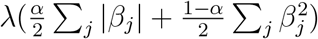 . The parameters α and λ are chosen by cross-validation. This constitutes a compromise between what is known as ridge regression (which is penalized by the ℓ2 norm,
  ), and LASSO (penalized by the ℓ1 norm,
  ). By including the ℓ1 norm in the penalty, elastic-net has the benefit of setting some coefficients to exactly 0, that is, selecting some variables while dropping others.
Finally, we construct a simple ensemble model in which each probability is a simple unweighted average of the probabilities produced by elastic-logit, rf, xgb, and krls. This has two primary benefits. The first is that such ensembles often have performance as good as the best sub-models and sometimes better. Second, it allows us to commit to reporting results for a single model—the ensemble model—as our premier estimate of the predictive power of these model on the test data. This is preferable to the tendency to choose the best-performing model on the test set, which can be misleading because such a choice is effectively a means of “training on the test set”.
Wealth model
Our wealth-based model employs wealth information flexibly: mortality is regressed on ten indicators for decile of wealth, equivalent to finding the mean mortality level in each wealth decide. In evaluating model performance, we can consider how being in the highest risk decile, quartile, or other groups is related to mortality risk. There is no presumption that risk is necessarily decreasing or even monotonic in the level of wealth.
We note that this is a wealth model, not a poverty model based on poverty assessments made by countries, usually based on income. Neither income nor poverty-assessments themselves are available in the DHS data. This limits our ability to benchmark against a true poverty-based system. That said, our wealth model may reasonably provide an optimistic indication of what can be predicted by income or poverty-based approaches. Household income is time-sensitive, but is likely to generate risks of early mortality when it remains low on average over a long period of time, in which case wealth will also drop. Moreover, financial shocks such as large expenses or losses may have little impact on income, but substantial impact on quality of life, access to healthcare, and poverty as locally understood (see e.g. Krishna, 2004). Our wealth model is also more flexible and less coarse than poverty-based targeting systems, which typically assign individuals through a binary system (e.g. above or below the poverty line).
Sample splitting and cross-validation
Before fitting each model, we split the data into training and test sets. For each country, 80% of observations are placed in a training and validation set, while 20% are retained in a held-out testing set. For the models described above, we tune hyperparameters using either 10-fold cross-validation within the training set (for elastic-logit, rf, xgb) or leave-one-out cross-validation (for krls). The cross-validation procedure also gives a preliminary assessment of model performance. Once all modeling choices were finalized based on this cross-validation, those models were “frozen” and we then assessed performance on the test set. This was done only once, after writing the bulk of the paper based on the cross-validation results, then updating the final values using the actual test-set results. This provides an honest assessment out-of-sample performance that prohibits “training on the test set”. We report the accuracy of the models using the performance metrics described below.
2.4 Performance metrics
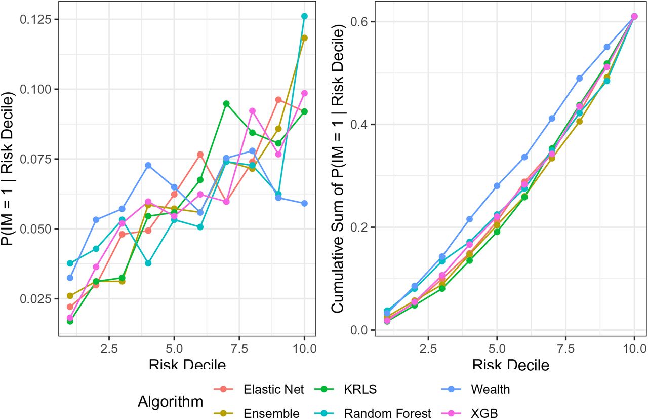
To evaluate our approach, we employ interpretable and policy-relevant metrics. A model’s recall (also referred to as sensitivity) is the proportion of actual deaths that are included in the group we consider to be at risk. What we term “recall10” is defined by first determining the group of births in the top risk decile (hence the “10”) according to our model, then computing the fraction of all actual infant deaths accounted for by this group. In policy terms, this corresponds to a case in which we have resources to target 10% of the population, and wish to know how much of the total mortality risk would be covered in that group. An ineffective risk assessment that assigns risk at random would produce a recall10 of 0.10 (10%). By contrast an effective system points us to a top risk decile that accounts for more than 10% of the mortality, perhaps 20% or 30%, for example. Similarly, we report recall20, which tells us the fraction of early deaths that occurred within the top risk quintile. For both recall10 and recall20, we also report “efficiency gain”, which tells us how many times more effective the ensemble model is than the benchmark wealth model.
2.4.1 Variable importance
Our models only seek to determine the best risk estimate possible given a set of predictors and the answers say nothing of the causal effect of those predictors on the risk of mortality. Indeed many of the risk factors, such as religion or the type of roof, are valuable not because they cause mortality but because they are expected to signal the presence of other, unobserved factors that cause higher mortality. In other words, confounding is expected and hoped for in these models.
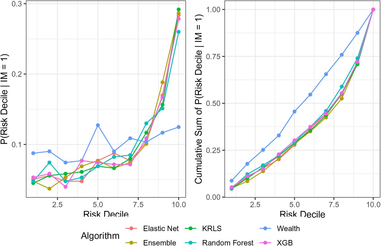
It is nevertheless of value to know what the models are doing to generate forecasts given the input variables. In particular we may wish to know which variables are most important in estimating the risk, for the purposes of assessing the credibility of the model or in focusing public health resources on data collection. Unfortunately, for many machine learning models it is more difficult to characterize what the model’s behavior than is the case with simpler regression approaches like OLS, in which the model is fully characterized by a small number of parameters. However, some tools are readily available and provide insights into the more and less important variables. Specifically, for elastic-net we report how often the model choose a given variable and the proportion of time their coefficient is positive. For random forest, the (scaled) “variable importance” describes what fraction of the time a given variable was chosen to be included in the classification trees over which each random forest model aggregates.
3 Results
The primary results are recall10 and recall20 rates computed on the held-out test set (Tables 2 and 3).1
recall10 results, test set
3.1 Poor performance of the wealth model
Table 2 shows the proportion of mortality that occurred among the top 10% highest predicted risk individuals. In Rwanda and Uganda, wealth is a reasonable indicator of risk, and the 10% of the population with the higher wealth-based predicted risk account for 24% and 18% of the mortality, respectively. In the other 20 countries, wealth is almost uninformative, with Recall10 values falling between just 3% (Tanzania) and 14% (Lesotho). Overall, the (country-wise) average recall10 of just 11% suggests that the wealth generally model does little or no better than chance in predicting which individuals are at highest risk.
Similarly, Table 3 shows that in most countries, recall20 is only slightly above 20%, averaging (country-wise) to 23%. Rwanda is again an exception, with the top quintile accounting for 48% of mortality, while recall20 rates range from 11% to 29% in the others, and are at or below chance (20%) in 9 of the 22 countries.
Recall20 results, test set
3.2 Beyond wealth: Gains from richer models
The elastic-net logit, rf, xgb, and krls all augment the wealth model by adding the additional variables described above. These models perform similarly to each other overall, and far better than the wealth-only model. The top risk deciles according to these models account for, on average, 17-20% of mortality (recall10); the top risk quintile accounts for 30-32% of mortality (recall20). The ensemble model performs better than any of the individual models, on average capturing 22% of the mortality in its top risk decile (recall10), and 35% in the top risk quintile (recall20). Compared to the wealth model, the ensemble model also captures 2.3 times as much of the mortality in its top risk decile (efficiency gain for recall10) and 1.6 times the mortality in its top risk quintile (efficiency gain for recall20). No single country always shows the highest recall10 across models, nor the lowest. Moreover, within given countries, the ensemble model outperforms the constituent models in many cases, does as well as the top one or two models in many others, and is never the worst performing model in that country. Thus, relying on the ensemble model not only yields better results than any other model on average, but also safeguards against cases where individual models perform poorly in a given country.
3.3 Variable selection
The elastic-net logistic regression model for each country automatically chooses a subset of variables to retain in the model, dropping the others. Surprisingly, every variable we provided was included in at least 36% of the country-level models. That is, at least taken across countries, there are not just a few key variables; rather the models tend to be fairly dense such that every variable is present in at least a third of the models. A few variables, though, are included especially often: most models included the previous death of a sibling in the first year (86%) or the death of any previous sibling at any point (76%). 77% of country level models included the child’s gender; 73% included an urban/rural indicator. Over two-thirds (68%) of models included the mother’s years of education, and many included the birth month (73% use sine-transformed birth month; 55% use cosine-transformed birth month). Maternal age was included in 64% of models.
For random forest, the “scaled variable importance” describes what fraction of the time a given variable was chosen to be included in the classification trees over which each random forest model aggregates. Compared to elastic-net logistic regression, random forest was somewhat more selective, with over half of variables appearing in fewer than 15% of the regression trees. A few variables were particularly rarely included, such as clean cooking fuel (3%) and minority religion (5%). By contrast, maternal age was included nearly every time (99.6%), followed closely by wealth percentile and it’s square (93%, 94%). The latter is particularly notable, as wealth percentiles were among the least commonly employed in the elastic-net logit models. Other important variables included malaria incidence rate in the area (92%), age of household head (77%), and mother’s age at first marriage or union (63%).
Variable Importance
4 Discussion
Across 22 countries in sub-Saharan Africa, predicting early mortality based on wealth measures alone was ineffective: those in highest 10% and 20% risk groups accounted for only 11% and 23% of mortality respectively. Fortunately, however, when wealth information is combined with other risk factors, flexible models can more accurately assess individual-level risk of early mortality. On average across countries, the 10% of births with the highest risk as predicted by the ensemble model account for 22% of deaths, and the 20% at highest risk account for 35%. Compared to the wealth-only models—which we expect are optimistic benchmarks for the poverty-based targeting approach—each country’s ensemble model on average would have identified 2.3 times as many deaths in the top risk decile, and 1.6 times as many in the top 20% risk group. Senegal offers a relatively representative example, in which targeting the poorest 10% will identify only 10% of all infant deaths, while targeting the 10% at highest risk according to the ensemble model would identify 29% of all deaths.
The various models used to incorporate these risk factors—a regularized logistic regression (elastic-logit), random forest (rf), extreme gradient boosting (xgb), and kernel regularized least squares (krls)—have similar average performance. However, some models exceed others in particular countries. Using the average of predictions from these (ensemble) generates better performance on average while importantly protecting against cases where individual models performed poorly in particular countries. Particularly important to many models were variables regarding the previous death of siblings in the first year, mother’s age and education, malaria prevalence, and the child’s gender. The value of these variables as predictors says nothing of their causal influence, and we often expect they are predictive because they signal the presence or absence of other, hard to measure factors that influence risk.
Central to the policy-relevance of such an approach is the question of whether the variables needed to run these models are generally accessible. The risk factors we included were all chosen to be feasibly collected and employed in targeting strategies by health agencies. We avoided post-birth variables, such as birth-weight, which require real-time data. Only the sex of the child and the calendar month of birth are unknown until the birth occurs, and this would not impeded the planning or siting of interventions and materials that are expected to reduce preventable deaths.
These findings are consistent with previous studies that show that births at high risk of death exist across all socioeconomic groups, and that combining multiple risk factors improves our ability to more accurately identify the higher risk births (Ramos et al., 2018, 2020; Houweling et al., 2019). Our findings are related to a large body of literature in medicine and public health that develops risk scores to identify those at risk of some event (e.g. Mpimbaza et al., 2015; Beymer et al., 2017). To our knowledge, prior work on infant mortality using flexible models or machine learning approaches had not previously been used to develop birth-level risk scores in sub-Saharan Africa.
How beneficial might this improvement in predictive power be? We consider the potential benefit of an improved targeting system such as this for a hypothetical intervention under resource constraints. Consider an intervention that a given country can afford to administer to only 10% of births. Ideally, this would be targeted to the 10% at highest risk of early mortality. This intervention would not reduce mortality among children who would not have died anyway, but let us suppose it reduces mortality by some proportion, efficacy, among those who would have otherwise have died. In a country with Nbirths per year, the number of lives saved per year would be efficacy ∗ P r(death|high risk) ∗ Nbirths/10. Applying Bayes’ rule, this is simply efficacy ∗ recall10 ∗ P r(death) ∗ Nbirths where P r(death) is the overall mortality rate expected for children born in that year (absent the intervention). Notice that the number of lives saved is proportional to the recall10 of the model used. Doubling the recall10—which is roughly what we see for all of our models compared to the wealth model—would double the lives saved by that intervention.
Using recent estimates of the number of births and baseline mortality rates in each of these countries from World Bank Development Indicators (2021), the number of lives saved by an intervention with efficacy = 5% would be 841 thousand for the wealth model, but 1.61 million for the ensemble model. In simpler terms, the efficiency gain of roughly two for these models compared to the wealth model translates into roughly double the lives saved by an intervention with any particular efficacy.2
We emphasize that all models here were trained and tuned by cross-validation on a training set, and the performance indicated here represents their performance on a test set that was completely unseen during training. If such models are to be used in practice, they would be retrained on the available data in a given country at present, but we emphasize the importance of careful tuning by cross-validation to avoid over-fitting that would lead to both over-confidence in the model’s ability and, quite possibly, poor performance in reality. That the results of our cross-validated models on the training set is nearly identical to the results on the test set, however, suggests that it is possible to estimate how well a model is likely to perform on as-yet unseen data if one is careful during the cross-validation procedure.
4.1 Limitations and Opportunities
Our work is not without limitations and indeed it explores the limits of machine learning methods to predict infant death risk. The first limitation of note is simply that not all deaths can be predicted, particularly with readily available data. In general we find our models for the highest 10% risk group capture only 20-30% of mortality. This is beneficial and worth using for targeting since the effectiveness of an intervention is proportional to this recall rate, as shown above. However, it leaves a great deal of unpredicted mortality spread across the lower risk groups. Thus, when possible, programs must still be targeted to a much wider group in order to capture a large fraction of births that will die.
Second, the DHS sampling procedure attempts to produce a sample that is representative of the population. If these are in fact not as representative as hoped, then while the results still reflect the predictive power of these models in some population of each country, the results may not be representative of these countries as a whole.
Third, the link between the improved predictive power of risk models and improved outcomes such as lives saved is complicated. While our simple hypothetical example above is intended only as an illustration, that exercise also reveals some of these complications. First, while the assumed the “efficacy” of a given hypothetical intervention is applied only to those individuals who would have otherwise have died, it is nevertheless possible that the even in this sense the true efficacy would not be constant across risk levels. For example, when children from wealthier families die young, it may less often be due to preventable causes, making the efficacy of any likely intervention lower. In our case this does little to jeopardize our finding: the efficacy rate need only apply to those in the top risk decile, and doing a poorer job of estimating risk would only further reduce the lives saved by reducing the effective efficacy. That is, accounting for this would only amplify the comparative benefits we describe of improved targeting. Second and more complicated, we are not incorporating targeting costs in our analysis. The calculus of the efficiency gains assumes that interventions have the same costs for each birth. In reality, costs need to be adjusted according to local conditions. For example, geographic location could be a major factor in calculating costs. Targeting children clustered by geographic location is likely much cheaper and easier than targeting children distant from each other, for example.
Finally, in the future this approach could be further improved if information of the cause of death were available. Associating each birth to a particular cause of the death could generate models that suggest targeting births with more specific, needed interventions.
Data Availability
The data is available via Demographic and Health Surveys.
A Appendix
A.1 Cross validation results
Recall10 results, cross-validation on training set
Recall20 results, cross-validation on training set
A.2 Variable construction
Variable information
B Online Supplement
B.1 Country-by-Country Results
Efficiency gain is measured by the ratio of Catch 10 Results for each algorithm compared to the Catch 10 Results for using wealth alone.
Detailed Results by Country
B.2 Angola
This sample was taken in the year 2015. There are 10829 observations in the dataset, and 8664 observations were used for the training set. Also, 195 observations were removed due to missing values. Finally, there were 472 deaths for the full dataset, and 378 deaths in the training set.
B.2.1 Variables Used
Variables included in the model for Angola
B.2.2 Mortality Breakdown by Wealth Quintile
B.2.3 Optimal Parameters
These are the algorithm parameters selected after cross-validation:
Optimal Parameters for the Elastic Net algorithm
Optimal Parameters for the Random Forest algorithm
Optimal Parameters for the XGB algorithm
Optimal Parameters for the KRLS algorithm
B.2.4 Table of Results
Manual Cross-Validation Results
Distribution of individuals in the top risk decile of each algorithm among each wealth decile
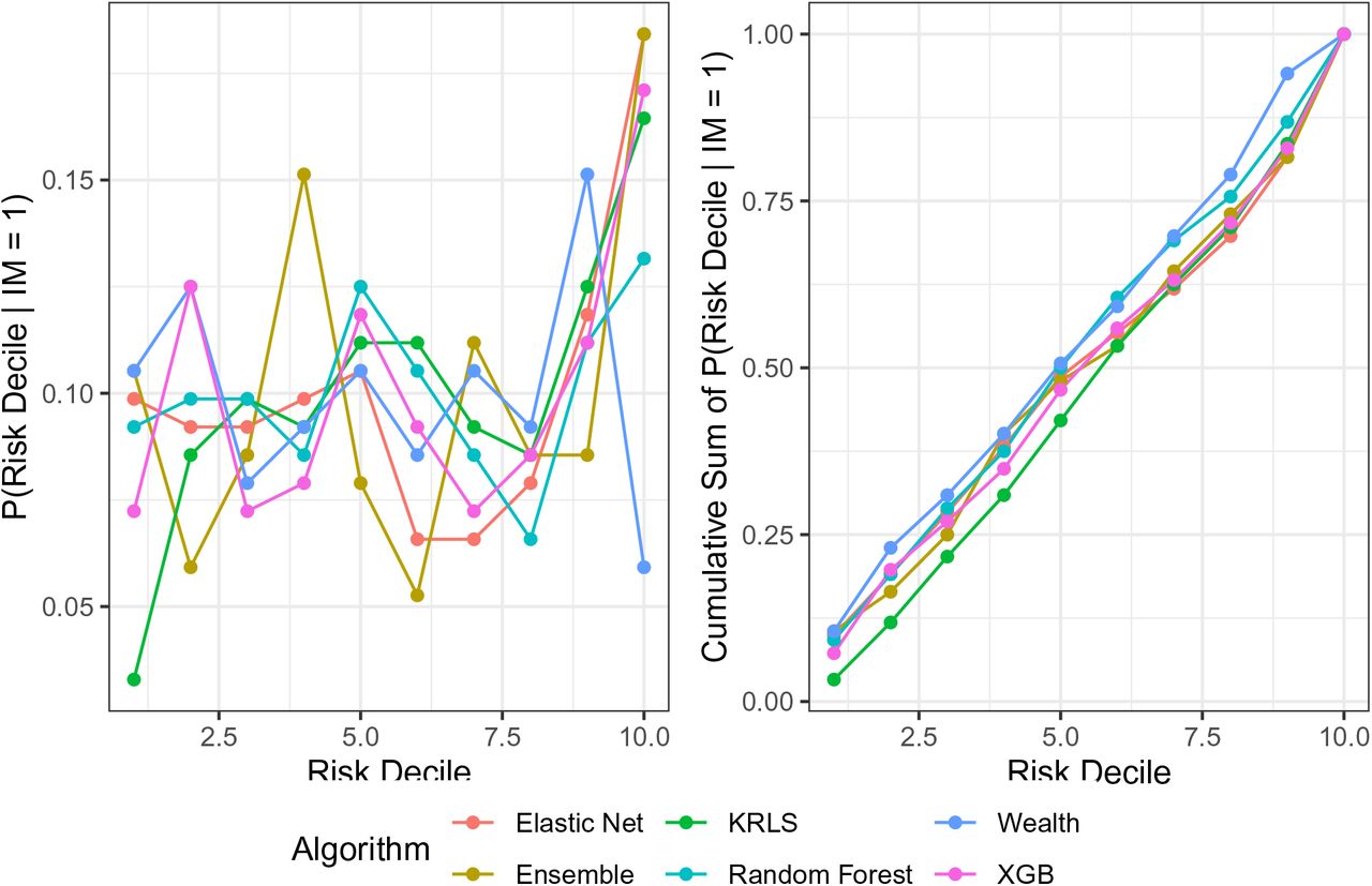
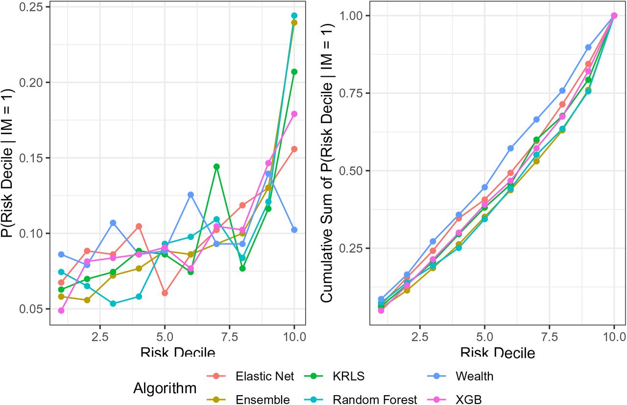
B.2.5 Performance Plots
Below are various plots showing the performance for each model considered in Angola.

Probability of a mortality given that the observation is in a particular risk decile

Probability of membership in a particular risk decile given a mortality

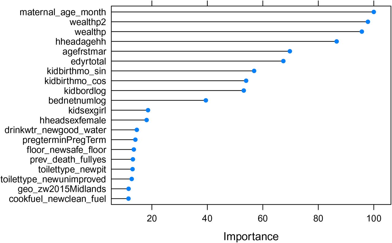
Variable Importance Plot generated by the Random Forest model
B.2.6 Variable Importance Plot
In this section we will show some measures to give some indication of the important variables necessary for predicting infant mortality.
B.2.7 Elastic Net Coefficients
Standardized coefficients from the optimal elastic net model after 10-fold cross-validation.
B.3 Benin
This sample was taken in the year 2011. There are 10199 observations in the dataset, and 8160 observations were used for the training set. Also, 291 observations were removed due to missing values. Finally, there were 471 deaths for the full dataset, and 377 deaths in the training set.
B.3.1 Variables Used
Variables included in the model for Benin
B.3.2 Mortality Breakdown by Wealth Quintile
B.3.3 Optimal Parameters
These are the algorithm parameters selected after cross-validation:
Optimal Parameters for the Elastic Net algorithm\
Optimal Parameters for the Random Forest algorithm
Optimal Parameters for the XGB algorithm\
Optimal Parameters for the KRLS algorithm
B.3.4 Table of Results
Manual Cross-Validation Results
Distribution of individuals in the top risk decile of each algorithm among each wealth decile
B.3.5 Performance Plots
Below are various plots showing the performance for each model considered in Benin.

Probability of a mortality given that the observation is in a particular risk decile
Probability of membership in a particular risk decile given a mortality

Variable Importance Plot generated by the Random Forest model
B.3.6 Variable Importance Plot
In this section we will show some measures to give some indication of the important variables necessary for predicting infant mortality.
B.3.7 Elastic Net Coefficients
Standardized coefficients from the optimal elastic net model after 10-fold cross-validation.
B.4 Burkina Faso
This sample was taken in the year 2010. There are 10905 observations in the dataset, and 8725 observations were used for the training set. Also, 823 observations were removed due to missing values. Finally, there were 752 deaths for the full dataset, and 602 deaths in the training set.
B.4.1 Variables Used
Variables included in the model for Burkina Faso
B.4.2 Mortality Breakdown by Wealth Quintile
B.4.3 Optimal Parameters
These are the algorithm parameters selected after cross-validation:
Optimal Parameters for the Elastic Net algorithm
Optimal Parameters for the Random Forest algorithm
Optimal Parameters for the XGB algorithm
Optimal Parameters for the KRLS algorithm
B.4.4 Table of Results
Manual Cross-Validation Results
Distribution of individuals in the top risk decile of each algorithm among each wealth decile
B.4.5 Performance Plots
Below are various plots showing the performance for each model considered in Burkina Faso.

Probability of a mortality given that the observation is in a particular risk decile

Probability of membership in a particular risk decile given a mortality
Variable Importance Plot generated by the Random Forest model
B.4.6 Variable Importance Plot
In this section we will show some measures to give some indication of the important variables necessary for predicting infant mortality.
B.4.7 Elastic Net Coefficients
Standardized coefficients from the optimal elastic net model after 10-fold cross-validation.
B.5 Cameroon
This sample was taken in the year 2011. There are 8450 observations in the dataset, and 6761 observations were used for the training set. Also, 591 observations were removed due to missing values. Finally, there were 564 deaths for the full dataset, and 452 deaths in the training set.
B.5.1 Variables Used
Variables included in the model for Cameroon
B.5.2 Mortality Breakdown by Wealth Quintile
B.5.3 Optimal Parameters
These are the algorithm parameters selected after cross-validation:
Optimal Parameters for the Elastic Net algorithm
Optimal Parameters for the Random Forest algorithm
Optimal Parameters for the XGB algorithm
Optimal Parameters for the KRLS algorithm
B.5.4 Table of Results
Manual Cross-Validation Results
Distribution of individuals in the top risk decile of each algorithm among each wealth decile
B.5.5 Performance Plots
Below are various plots showing the performance for each model considered in Cameroon.

Probability of a mortality given that the observation is in a particular risk decile

Probability of membership in a particular risk decile given a mortality

Variable Importance Plot generated by the Random Forest model
B.5.6 Variable Importance Plot
In this section we will show some measures to give some indication of the important variables necessary for predicting infant mortality.
B.5.7 Elastic Net Coefficients
Standardized coefficients from the optimal elastic net model after 10-fold cross-validation.
B.6 Cote d’Ivoire
This sample was taken in the year 2011. There are 5211 observations in the dataset, and 4169 observations were used for the training set. Also, 734 observations were removed due to missing values. Finally, there were 421 deaths for the full dataset, and 337 deaths in the training set.
B.6.1 Variables Used
Variables included in the model for Cote d’Ivoire
B.6.2 Mortality Breakdown by Wealth Quintile
B.6.3 Optimal Parameters
These are the algorithm parameters selected after cross-validation:
Optimal Parameters for the Elastic Net algorithm
Optimal Parameters for the Random Forest algorithm
Optimal Parameters for the XGB algorithm
Optimal Parameters for the KRLS algorithm
B.6.4 Table of Results
Manual Cross-Validation Results
Distribution of individuals in the top risk decile of each algorithm among each wealth decile
B.6.5 Performance Plots
Below are various plots showing the performance for each model considered in Cote d’Ivoire.

Probability of a mortality given that the observation is in a particular risk decile

Probability of membership in a particular risk decile given a mortality

Variable Importance Plot generated by the Random Forest model
B.6.6 Variable Importance Plot
In this section we will show some measures to give some indication of the important variables necessary for predicting infant mortality.
B.6.7 Elastic Net Coefficients
Standardized coefficients from the optimal elastic net model after 10-fold cross-validation.
B.7 Ghana
This sample was taken in the year 2014. There are 4203 observations in the dataset, and 3364 observations were used for the training set. Also, 345 observations were removed due to missing values. Finally, there were 189 deaths for the full dataset, and 152 deaths in the training set.
B.7.1 Variables Used
Variables included in the model for Ghana
B.7.2 Mortality Breakdown by Wealth Quintile
B.7.3 Optimal Parameters
These are the algorithm parameters selected after cross-validation:
Optimal Parameters for the Elastic Net algorithm
Optimal Parameters for the Random Forest algorithm
Optimal Parameters for the XGB algorithm
Optimal Parameters for the KRLS algorithm
B.7.4 Table of Results
Manual Cross-Validation Results
Distribution of individuals in the top risk decile of each algorithm among each wealth decile
B.7.5 Performance Plots
Below are various plots showing the performance for each model considered in Ghana.

Probability of a mortality given that the observation is in a particular risk decile

Probability of membership in a particular risk decile given a mortality

Variable Importance Plot generated by the Random Forest model
B.7.6 Variable Importance Plot
In this section we will show some measures to give some indication of the important variables necessary for predicting infant mortality.
B.7.7 Elastic Net Coefficients
Standardized coefficients from the optimal elastic net model after 10-fold cross-validation.
B.8 Guinea
This sample was taken in the year 2012. There are 5223 observations in the dataset, and 4179 observations were used for the training set. Also, 199 observations were removed due to missing values. Finally, there were 396 deaths for the full dataset, and 317 deaths in the training set.
B.8.1 Variables Used
Variables included in the model for Guinea
B.8.2 Mortality Breakdown by Wealth Quintile
B.8.3 Optimal Parameters
These are the algorithm parameters selected after cross-validation:
Optimal Parameters for the Elastic Net algorithm
Optimal Parameters for the Random Forest algorithm
Optimal Parameters for the XGB algorithm
Optimal Parameters for the KRLS algorithm
B.8.4 Table of Results
Manual Cross-Validation Results
Distribution of individuals in the top risk decile of each algorithm among each wealth decile
B.8.5 Performance Plots
Below are various plots showing the performance for each model considered in Guinea.

Probability of a mortality given that the observation is in a particular risk decile

Probability of membership in a particular risk decile given a mortality

Variable Importance Plot generated by the Random Forest model
B.8.6 Variable Importance Plot
In this section we will show some measures to give some indication of the important variables necessary for predicting infant mortality.
B.8.7 Elastic Net Coefficients
Standardized coefficients from the optimal elastic net model after 10-fold cross-validation.
B.9 Kenya
This sample was taken in the year 2014. There are 15110 observations in the dataset, and 12089 observations were used for the training set. Also, 1447 observations were removed due to missing values. Finally, there were 589 deaths for the full dataset, and 472 deaths in the training set.
B.9.1 Variables Used
Variables included in the model for Kenya
B.9.2 Mortality Breakdown by Wealth Quintile
B.9.3 Optimal Parameters
These are the algorithm parameters selected after cross-validation:
Optimal Parameters for the Elastic Net algorithm
Optimal Parameters for the Random Forest algorithm
Optimal Parameters for the XGB algorithm
Optimal Parameters for the KRLS algorithm
B.9.4 Table of Results
Manual Cross-Validation Results
Distribution of individuals in the top risk decile of each algorithm among each wealth decile
B.9.5 Performance Plots
Below are various plots showing the performance for each model considered in Kenya.

Probability of a mortality given that the observation is in a particular risk decile

Probability of membership in a particular risk decile given a mortality

Variable Importance Plot generated by the Random Forest model
B.9.6 Variable Importance Plot
In this section we will show some measures to give some indication of the important variables necessary for predicting infant mortality.
B.9.7 Elastic Net Coefficients
Standardized coefficients from the optimal elastic net model after 10-fold cross-validation.
B.10 Lesotho
This sample was taken in the year 2014. There are 2127 observations in the dataset, and 1702 observations were used for the training set. Also, 233 observations were removed due to missing values. Finally, there were 145 deaths for the full dataset, and 116 deaths in the training set.
B.10.1 Variables Used
Variables included in the model for Lesotho
B.10.2 Mortality Breakdown by Wealth Quintile
B.10.3 Optimal Parameters
These are the algorithm parameters selected after cross-validation:
Optimal Parameters for the Elastic Net algorithm
Optimal Parameters for the Random Forest algorithm
Optimal Parameters for the XGB algorithm
Optimal Parameters for the KRLS algorithm
B.10.4 Table of Results
Manual Cross-Validation Results
Distribution of individuals in the top risk decile of each algorithm among each wealth decile
B.10.5 Performance Plots
Below are various plots showing the performance for each model considered in Lesotho.

Probability of a mortality given that the observation is in a particular risk decile

Probability of membership in a particular risk decile given a mortality

Variable Importance Plot generated by the Random Forest model
B.10.6 Variable Importance Plot
In this section we will show some measures to give some indication of the important variables necessary for predicting infant mortality.
B.10.7 Elastic Net Coefficients
Standardized coefficients from the optimal elastic net model after 10-fold cross-validation.
B.11 Madagascar
This sample was taken in the year 2008. There are 9229 observations in the dataset, and 7384 observations were used for the training set. Also, 428 observations were removed due to missing values. Finally, there were 459 deaths for the full dataset, and 368 deaths in the training set.
B.11.1 Variables Used
Variables included in the model for Madagascar
B.11.2 Mortality Breakdown by Wealth Quintile
B.11.3 Optimal Parameters
These are the algorithm parameters selected after cross-validation:
Optimal Parameters for the Elastic Net algorithm
Optimal Parameters for the Random Forest algorithm
Optimal Parameters for the XGB algorithm
Optimal Parameters for the KRLS algorithm
B.11.4 Table of Results
Manual Cross-Validation Results
Distribution of individuals in the top risk decile of each algorithm among each wealth decile
B.11.5 Performance Plots
Below are various plots showing the performance for each model considered in Madagascar.

Probability of a mortality given that the observation is in a particular risk decile

Probability of membership in a particular risk decile given a mortality

Variable Importance Plot generated by the Random Forest model
B.11.6 Variable Importance Plot
In this section we will show some measures to give some indication of the important variables necessary for predicting infant mortality.
B.11.7 Elastic Net Coefficients
Standardized coefficients from the optimal elastic net model after 10-fold cross-validation.
B.12 Malawi
This sample was taken in the year 2016. There are 13231 observations in the dataset, and 10586 observations were used for the training set. Also, 402 observations were removed due to missing values. Finally, there were 563 deaths for the full dataset, and 451 deaths in the training set.
B.12.1 Variables Used
Variables included in the model for Malawi
B.12.2 Mortality Breakdown by Wealth Quintile
B.12.3 Optimal Parameters
These are the algorithm parameters selected after cross-validation:
Optimal Parameters for the Elastic Net algorithm
Optimal Parameters for the Random Forest algorithm
Optimal Parameters for the XGB algorithm
Optimal Parameters for the KRLS algorithm
B.12.4 Table of Results
Manual Cross-Validation Results
Distribution of individuals in the top risk decile of each algorithm among each wealth decile
B.12.5 Performance Plots
Below are various plots showing the performance for each model considered in Malawi.

Probability of a mortality given that the observation is in a particular risk decile

Probability of membership in a particular risk decile given a mortality

Variable Importance Plot generated by the Random Forest model
B.12.6 Variable Importance Plot
In this section we will show some measures to give some indication of the important variables necessary for predicting infant mortality.
B.12.7 Elastic Net Coefficients
Standardized coefficients from the optimal elastic net model after 10-fold cross-validation.
B.13 Mali
This sample was taken in the year 2012. There are 7913 observations in the dataset, and 6331 observations were used for the training set. Also, 130 observations were removed due to missing values. Finally, there were 475 deaths for the full dataset, and 380 deaths in the training set.
B.13.1 Variables Used
Variables included in the model for Mali
B.13.2 Mortality Breakdown by Wealth Quintile
B.13.3 Optimal Parameters
These are the algorithm parameters selected after cross-validation:
Optimal Parameters for the Elastic Net algorithm
Optimal Parameters for the Random Forest algorithm
Optimal Parameters for the XGB algorithm
Optimal Parameters for the KRLS algorithm
B.13.4 Table of Results
Manual Cross-Validation Results
Distribution of individuals in the top risk decile of each algorithm among each wealth decile
B.13.5 Performance Plots
Below are various plots showing the performance for each model considered in Mali.

Probability of a mortality given that the observation is in a particular risk decile

Probability of membership in a particular risk decile given a mortality

Variable Importance Plot generated by the Random Forest model
B.13.6 Variable Importance Plot
In this section we will show some measures to give some indication of the important variables necessary for predicting infant mortality.
B.13.7 Elastic Net Coefficients
Standardized coefficients from the optimal elastic net model after 10-fold cross-validation.
B.14 Mozambique
This sample was taken in the year 2011. There are 8026 observations in the dataset, and 6422 observations were used for the training set. Also, 467 observations were removed due to missing values. Finally, there were 537 deaths for the full dataset, and 430 deaths in the training set.
B.14.1 Variables Used
Variables included in the model for Mozambique
B.14.2 Mortality Breakdown by Wealth Quintile
B.14.3 Optimal Parameters
These are the algorithm parameters selected after cross-validation:
Optimal Parameters for the Elastic Net algorithm
Optimal Parameters for the Random Forest algorithm
Optimal Parameters for the XGB algorithm
Optimal Parameters for the KRLS algorithm
B.14.4 Table of Results
Manual Cross-Validation Results
Distribution of individuals in the top risk decile of each algorithm among each wealth decile
B.14.5 Performance Plots
Below are various plots showing the performance for each model considered in Mozambique.

Probability of a mortality given that the observation is in a particular risk decile

Probability of membership in a particular risk decile given a mortality

Variable Importance Plot generated by the Random Forest model
B.14.6 Variable Importance Plot
In this section we will show some measures to give some indication of the important variables necessary for predicting infant mortality.
B.14.7 Elastic Net Coefficients
Standardized coefficients from the optimal elastic net model after 10-fold cross-validation.
B.15 Niger
This sample was taken in the year 2012. There are 9612 observations in the dataset, and 7690 observations were used for the training set. Also, 38 observations were removed due to missing values. Finally, there were 586 deaths for the full dataset, and 469 deaths in the training set.
B.15.1 Variables Used
Variables included in the model for Niger
B.15.2 Mortality Breakdown by Wealth Quintile
B.15.3 Optimal Parameters
These are the algorithm parameters selected after cross-validation:
Optimal Parameters for the Elastic Net algorithm
Optimal Parameters for the Random Forest algorithm
Optimal Parameters for the XGB algorithm
Optimal Parameters for the KRLS algorithm
B.15.4 Table of Results
Manual Cross-Validation Results
Distribution of individuals in the top risk decile of each algorithm among each wealth decile
B.15.5 Performance Plots
Below are various plots showing the performance for each model considered in Niger.
Probability of a mortality given that the observation is in a particular risk decile

Probability of membership in a particular risk decile given a mortality

Variable Importance Plot generated by the Random Forest model
B.15.6 Variable Importance Plot
In this section we will show some measures to give some indication of the important variables necessary for predicting infant mortality.
B.15.7 Elastic Net Coefficients
Standardized coefficients from the optimal elastic net model after 10-fold cross-validation.
B.16 Nigeria
This sample was taken in the year 2013. There are 23559 observations in the dataset, and 18848 observations were used for the training set. Also, 663 observations were removed due to missing values. Finally, there were 1686 deaths for the full dataset, and 1349 deaths in the training set.
B.16.1 Variables Used
Variables included in the model for Nigeria
B.16.2 Mortality Breakdown by Wealth Quintile
B.16.3 Optimal Parameters
These are the algorithm parameters selected after cross-validation:
Optimal Parameters for the Elastic Net algorithm
Optimal Parameters for the Random Forest algorithm
Optimal Parameters for the XGB algorithm
Optimal Parameters for the KRLS algorithm
B.16.4 Table of Results
Manual Cross-Validation Results
Distribution of individuals in the top risk decile of each algorithm among each wealth decile
B.16.5 Performance Plots
Below are various plots showing the performance for each model considered in Nigeria.

Probability of a mortality given that the observation is in a particular risk decile

Probability of membership in a particular risk decile given a mortality

Variable Importance Plot generated by the Random Forest model
B.16.6 Variable Importance Plot
In this section we will show some measures to give some indication of the important variables necessary for predicting infant mortality.
B.16.7 Elastic Net Coefficients
Standardized coefficients from the optimal elastic net model after 10-fold cross-validation.
B.17 Rwanda
This sample was taken in the year 2014. There are 5350 observations in the dataset, and 4281 observations were used for the training set. Also, 705 observations were removed due to missing values. Finally, there were 168 deaths for the full dataset, and 135 deaths in the training set.
B.17.1 Variables Used
Variables included in the model for Rwanda
B.17.2 Mortality Breakdown by Wealth Quintile
B.17.3 Optimal Parameters
These are the algorithm parameters selected after cross-validation:
Optimal Parameters for the Elastic Net algorithm
Optimal Parameters for the Random Forest algorithm
Optimal Parameters for the XGB algorithm
Optimal Parameters for the KRLS algorithm
B.17.4 Table of Results
Manual Cross-Validation Results
Distribution of individuals in the top risk decile of each algorithm among each wealth decile
B.17.5 Performance Plots
Below are various plots showing the performance for each model considered in Rwanda.

Probability of a mortality given that the observation is in a particular risk decile

Probability of membership in a particular risk decile given a mortality

Variable Importance Plot generated by the Random Forest model
B.17.6 Variable Importance Plot
In this section we will show some measures to give some indication of the important variables necessary for predicting infant mortality.
B.17.7 Elastic Net Coefficients
Standardized coefficients from the optimal elastic net model after 10-fold cross-validation.
B.18 Senegal
This sample was taken in the year 2017. There are 9371 observations in the dataset, and 7497 observations were used for the training set. Also, 214 observations were removed due to missing values. Finally, there were 401 deaths for the full dataset, and 321 deaths in the training set.
B.18.1 Variables Used
Variables included in the model for Senegal
B.18.2 Mortality Breakdown by Wealth Quintile
B.18.3 Optimal Parameters
These are the algorithm parameters selected after cross-validation:
Optimal Parameters for the Elastic Net algorithm
Optimal Parameters for the Random Forest algorithm
Optimal Parameters for the XGB algorithm
Optimal Parameters for the KRLS algorithm
B.18.4 Table of Results
Manual Cross-Validation Results
Distribution of individuals in the top risk decile of each algorithm among each wealth decile
B.18.5 Performance Plots
Below are various plots showing the performance for each model considered in Senegal.

Probability of a mortality given that the observation is in a particular risk decile

Probability of membership in a particular risk decile given a mortality

Variable Importance Plot generated by the Random Forest model
B.18.6 Variable Importance Plot
In this section we will show some measures to give some indication of the important variables necessary for predicting infant mortality.
B.18.7 Elastic Net Coefficients
Standardized coefficients from the optimal elastic net model after 10-fold cross-validation.
B.19 Tanzania
This sample was taken in the year 2015. There are 7688 observations in the dataset, and 6152 observations were used for the training set. Also, 319 observations were removed due to missing values. Finally, there were 319 deaths for the full dataset, and 256 deaths in the training set.
B.19.1 Variables Used
Variables included in the model for Tanzania
B.19.2 Mortality Breakdown by Wealth Quintile
B.19.3 Optimal Parameters
These are the algorithm parameters selected after cross-validation:
Optimal Parameters for the Elastic Net algorithm
Optimal Parameters for the Random Forest algorithm
Optimal Parameters for the XGB algorithm
Optimal Parameters for the KRLS algorithm
B.19.4 Table of Results
Manual Cross-Validation Results
Distribution of individuals in the top risk decile of each algorithm among each wealth decile
B.19.5 Performance Plots
Below are various plots showing the performance for each model considered in Tanzania.

Probability of a mortality given that the observation is in a particular risk decile

Probability of membership in a particular risk decile given a mortality

Variable Importance Plot generated by the Random Forest model
B.19.6 Variable Importance Plot
In this section we will show some measures to give some indication of the important variables necessary for predicting infant mortality.
B.19.7 Elastic Net Coefficients
Standardized coefficients from the optimal elastic net model after 10-fold cross-validation.
B.20 Uganda
This sample was taken in the year 2016. There are 11619 observations in the dataset, and 9296 observations were used for the training set. Also, 470 observations were removed due to missing values. Finally, there were 484 deaths for the full dataset, and 388 deaths in the training set.
B.20.1 Variables Used
Variables included in the model for Uganda
B.20.2 Mortality Breakdown by Wealth Quintile
B.20.3 Optimal Parameters
These are the algorithm parameters selected after cross-validation:
Optimal Parameters for the Elastic Net algorithm
Optimal Parameters for the Random Forest algorithm
Optimal Parameters for the XGB algorithm
Optimal Parameters for the KRLS algorithm
B.20.4 Table of Results
Manual Cross-Validation Results
Distribution of individuals in the top risk decile of each algorithm among each wealth decile
B.20.5 Performance Plots
Below are various plots showing the performance for each model considered in Uganda.

Probability of a mortality given that the observation is in a particular risk decile

Probability of membership in a particular risk decile given a mortality

Variable Importance Plot generated by the Random Forest model
B.20.6 Variable Importance Plot
In this section we will show some measures to give some indication of the important variables necessary for predicting infant mortality.
B.20.7 Elastic Net Coefficients
Standardized coefficients from the optimal elastic net model after 10-fold cross-validation.
B.21 Zambia
This sample was taken in the year 2013. There are 9811 observations in the dataset, and 7850 observations were used for the training set. Also, 835 observations were removed due to missing values. Finally, there were 483 deaths for the full dataset, and 387 deaths in the training set.
B.21.1 Variables Used
Variables included in the model for Zambia
B.21.2 Mortality Breakdown by Wealth Quintile
B.21.3 Optimal Parameters
These are the algorithm parameters selected after cross-validation:
Optimal Parameters for the Elastic Net algorithm
Optimal Parameters for the Random Forest algorithm
Optimal Parameters for the XGB algorithm
Optimal Parameters for the KRLS algorithm
B.21.4 Table of Results
Manual Cross-Validation Results
Distribution of individuals in the top risk decile of each algorithm among each wealth decile
B.21.5 Performance Plots
Below are various plots showing the performance for each model considered in Zambia.

Probability of a mortality given that the observation is in a particular risk decile

Probability of membership in a particular risk decile given a mortality

Variable Importance Plot generated by the Random Forest model
B.21.6 Variable Importance Plot
In this section we will show some measures to give some indication of the important variables necessary for predicting infant mortality.
B.21.7 Elastic Net Coefficients
Standardized coefficients from the optimal elastic net model after 10-fold cross-validation.
B.22 Zimbabwe
This sample was taken in the year 2015. There are 4630 observations in the dataset, and 3705 observations were used for the training set. Also, 222 observations were removed due to missing values. Finally, there were 236 deaths for the full dataset, and 189 deaths in the training set.
B.22.1 Variables Used
Variables included in the model for Zimbabwe
B.22.2 Mortality Breakdown by Wealth Quintile
B.22.3 Optimal Parameters
These are the algorithm parameters selected after cross-validation:
Optimal Parameters for the Elastic Net algorithm
Optimal Parameters for the Random Forest algorithm
Optimal Parameters for the XGB algorithm
Optimal Parameters for the KRLS algorithm
B.22.4 Table of Results
Manual Cross-Validation Results
Distribution of individuals in the top risk decile of each algorithm among each wealth decile
B.22.5 Performance Plots
Below are various plots showing the performance for each model considered in Zimbabwe.

Probability of a mortality given that the observation is in a particular risk decile

Probability of membership in a particular risk decile given a mortality

Variable Importance Plot generated by the Random Forest model
B.22.6 Variable Importance Plot
In this section we will show some measures to give some indication of the important variables necessary for predicting infant mortality.
B.22.7 Elastic Net Coefficients
Standardized coefficients from the optimal elastic net model after 10-fold cross-validation.
Footnotes
chazlett{at}ucla.edu URL: http://www.chadhazlett.com, Email: stephensmith13424{at}gmail.com
↵1 Appendix A.1 provides the same performance metrics, but using cross-validated results from the training set. Those results are extremely similar to the test set results reported here, indicating very little over-fitting in the training process.
↵2 Note that the average efficiency gain (2.3) is not exactly the ratio of lives saved because the latter takes the relative birth rates and mortality in each country into account.


