
ABSTRACT
Short-term reattendances to emergency departments are a key quality of care indicator. Identifying patients at increased risk of early reattendance can help reduce the number of patients with missed or undertreated illness or injury, and could support appropriate discharges with focused interventions. In this manuscript we present a retrospective, single-centre study where we create and evaluate a machine-learnt classifier trained to identify patients at risk of reattendance within 72 hours of discharge from an emergency department. On a patient hold-out test set, our highest performing classifier obtained an AUROC of 0.748 and an average precision of 0.250; demonstrating that machine-learning algorithms can be used to classify patients, with moderate performance, into low and high-risk groups for reattendance. In parallel to our predictive model we train an explanation model, capable of explaining predictions at an attendance level, which can be used to help inform the design of interventional strategies.
Introduction
The demand for emergency departments (EDs) has been growing steadily over the last decade1,2, which in turn has contributed to increased overcrowding and extended waiting times. Since delays in care and overcrowding have been linked to increased rates of adverse outcomes3,4, it is important to investigate the most efficient ways of using the available resources and, importantly, minimise and mitigate their unnecessary use. Short-term reattendances describe the situation whereby a patient attends an emergency department (ED) within 72 hours of having been discharged. This reattendance rate will include patients with missed or undertreated illness, attendance with a new injury/illness, as well as scheduled reattendance for clinical review following an injury. Focused interventions could reduce inappropriate discharges as well as support patients at home, reducing subsequent reattendance.
Research has shown there are several factors indicative of short-term reattendance risk including social factors (e.g., living alone)5, depression6, initial diagnosis7, and historical emergency department usage8. Knowledge of these risk factors is important to clinical staff when planning discharge, but this is unlikely the most optimal way of determining those at risk of suffering from a significant illness following erroneous discharge or those in need of additional support in the community following discharge from an ED. Predictive models, available as a decision support tool at the point of discharge, able to reliably identify those at increased risk of short-term reattendance using known risk factors and attendance level information, may be able to significantly reduce the number of reattendances by appropriately quantifying and explaining a patient’s risk of reattendance to clinical staff. Ultimately this would allow appropriate focussed interventions (e.g., further diagnostic tests), more informed discussions about a patients discharge plan, or support in the community for those recently discharged.
Machine learnt models are a class of predictive models which are particularly well positioned to add value to emergency department processes. By making use of large amounts of clinical and administrative data, these models can provide estimates of a patient’s short-term reattendance risk9,10and explain the reason for the patient’s predicted risk. Explanation is particularly important, as this could help either inform the patient care trajectory or guide the post-discharge intervention plan. In this manuscript we discuss a machine-learnt model, utilizing data extracted from historical (coded, inpatient) discharge summaries, alongside contemporary attendance recorded clinical data such as observations and results of standard triage processes, to identify patients at increased risk of short-term reattendance following an emergency department attendance. In addition to our predictive model, we construct an explanation model which allow us to evaluate the trends our model has learned and explain our model’s prediction at an attendance level.
Methods
Dataset curation
The dataset features a pseudonymized version of all attendances by adults to Southampton’s Emergency Department (University Hospitals Southampton Foundation Trust) occurring between the 1st April 2019 and the 30th of April 2020. For our study cohort, we take only attendances which resulted in discharge directly from the ED, of which there were 54,021. The core dataset includes patients’ year of birth, results of any near-patient observations recorded, and high-level information about the attendance included in the standard UK Emergency Care Data Set (ECDS, which maps to SNOMED CT diagnostic codes). The data was prospectively digitally recorded within the ED electronic patient record (EMIS Symphony). To provide the machine learning classifier with a view of patients’ medical history we make use of historical discharge summaries associated with the patient, both from the emergency department and from the patients electronic health record maintained by the University Hospitals Southampton Foundation Trust. For a given patient, from any discharge summary occurring prior to a given emergency department attendance, we make use of ICD10 coded conditions (e.g., type 2 diabetes, current smoker) and create a binary indicator which indicates whether a patient has a given condition coded in their electronic health record prior to a given ED attendance. The electronic health records used by our models are available to review by clinicians and are used in regular practice. Our model does not have access to any free text fields in the electronic health record. Previous studies have shown that (free text) clinical notes can be predictive of patient outcomes across the broader hospital network11,12, but including these notes was beyond the scope of our study as they would limit the explainability of our algorithms. An example of the most frequently observed conditions are presented in Table 1.
The left column denotes the noted conditions (as specified by ICD10 codes) and the right column the number of attendances in the training set noted to have this condition. A given condition is only associated with a small fraction of attendances, but in total 38.9 % of attendances resulting in discharge have at least one associated condition. Conditions are generated by extracting from the (ICD10) coded discharge sumaaries held in a patients electronic health record.
Reattendance identification
Patient reattendances are identified by using the patient pseudo identifier to calculate the time to their next ED attendance. Importantly, all reattendances are considered, even if the second attendance is for a different condition to the original attendance (see Supplementary Figure 2 for further details). This is then dichotomized (less than 72 hours) to annotate each attendance with whether the discharge was followed by another attendance by the same patient within 72 hours. This formulation allowed us to frame the predictive task as a binary classification problem.

Discarded attendances were those that occurred in either the first 30 days or last 72 hours of the temporal test, to avoid information leakage between the training and temporal test set and because the reattendance status could not be robustly calculated for attendances occurring in the last 72 hours of the dataset. Reattendance rates (bottom row of shaded boxes) display the observed 72-hour reattendance rate for each cohort.

a) Receiving operator curve for model’s prediction. b) Precision recall curve for predictions on test set, the dashed grey line shows the configuration evaluated in the confusion matrix in panel c. c) Confusion matrix for predictions dichotomized using a threshold chosen such that the recall is equal to 0.15 (dashed grey line in panel b). A class of ‘1’ indicates the patient reattended the emergency department within 72 hours of discharge. Diagonal elements represent correct classifications and off-diagonal elemements either False positives or negatives.
Predictive modelling
We separated our data into a training set and two independent test sets (Figure 1). The last 3 months of attendances (01/02/2020 to 30/04/2020, inclusive of the COVID-19 pandemic) were segregated as a temporal test set, excluding any visit which took part in either the first 30 days or the final 72 hours. These exclusions remove information leakage between the training and temporal test set and attendances where reattendance to the emergency department could not be calculated reliably (i.e., those occuring in the last 72 hours of the data extract). The remaining attendances (N=44,857) were randomly split at the patient level to create a patient-level hold test set containing attendances from 20 % of the remaining patients. Remaining attendances (N=35,645) were used as the training and validation set. The number of patients in each respective dataset was 4,458, 7,238, and 28,951. The relation between patients in each dataset is displayed in Supplementary Figure 1, demonstrating patient exclusivity between the training set and the patient hold-out test set. The temporal test set is discussed in the Supplementary Information only.
Metrics are evaluated on the training set using grouped 5-fold CV at the patient level and we report the mean of the metric across the five validation folds. All models hyperparameters were tuned as described in the methods section to optimize the CV AUROC.
As our machine-learnt classifier, we used a gradient boosted decision tree as implemented in the XGBoost framework16. Features used in modelling include : patient age (estimated from year of birth), number of emergency department attendances in the 30 days prior to the attendance, the chief complaint of the attendance (e.g., ‘abdominal pain’), the patients mode of arrival, previously described medical condition indicators, the count of the number of medical conditions a patient has, vital signs (temperature, pulse and respiration rate, systolic blood pressure, and blood oxygen saturation levels), the Manchester Triage System score, triage pain score, (coded) discharge diagnosis, and the hour of day and day of the week the attendance occurred. A full data schema is presented in Supplementary Table 1. Medical conditions associated with the patient at a given attendance were included as a one-hot-encoded feature vector, the day of the week encoded using ordinal encoding, and all other categorical variables were encoded using target encoding13. Hyperparameters were tuning using five-fold cross-validation (CV) of the training set at the patient level (the set of attendances from a unique patient appear exclusively in validation or training for each fold) using Bayesian optimization utilizing the Tree Parzen Estimator algorithm as implemented in the hyperopt Python library14,15. Feature selection was performed using a greedy, sequential forward selection approach. Starting with the single most predictive variable (as determined by the CV score of a model trained with a single variable only) we added another variable to the feature set, where the variable added selected was the one which increased the CV score by the largest amount. We sequentially added variables to the feature set in this manner until all variables were included in the feature set. The optimal feature set for our final model was selected by the set that yielded the highest CV score (Supplementary Table 2).
We evaluate our final model performance (the average output of the five models trained during cross-validation) on the two hold-out test sets. Models performance is evaluated using the Area Under the Receiving Operating Curve (AUROC) and the average precision under the precision-recall curve.
Model explainability
To explain the predictions of our model we make use of the TreeExplainer algorithm in the SHAP Python library17–19. TreeExplainer calculates SHAP values (i.e, Shapley values), a concept from coalitional game theory which treats predictive variables as players in a game and distributes their contribution to the predicted probability. To calculate the SHAP value for a given feature, one trains a model for each possible feature set (with and without the given feature) and calculates the mean change in the predicted probability when the feature was added to a feature set for all possible sets of features. This mean change is the SHAP value and can be negative (adding the feature predicted reduces reattendance risk) or positive (adding the feature increases the predicted reattendance risk). SHAP values are particularly powerful as they meet the four desirable theoretical conditions of an explanation algorithm and can provide instance (i.e., attendance) level explanations19. Practically, for each attendance we will have a scalar value for each variable used in the model which quantifies the contribution that variable had on the predicted reattendance risk for the given attendance, with SHAP values of larger magnitudes indicating that the relevant variable was more significant in determining the predicted reattendance risk.
To investigate the different explanations across the whole dataset, we project the SHAP values for all attendances into a two-dimensional (‘explanation’) space using Uniform Manifold Approximation and Projection (UMAP)20. UMAP is a dimensionality reduction technique regularly used to visualise high-dimensional spaces in a low-dimensional embedding, such that global and local structure of the space can be explored21,22. Attendances which are closer in proximity in this two-dimensional space share a similar explanation for their predicted reattendance risk.
Ethics and data governance
This study was approved by the University of Southampton’s Ethics and Research governance committee (ERGO/FEPS/53164) and approval was obtained from the Health Research Authority (20/HRA/1102). Data was pseudonymized (and where appropriate linked) before being passed to the research team. The research team did not have access to the pseudonymisation key.
Results
To investigate the potential of individual variables and sets of variables at predicting 72-hour reattendance we constructed a series of XGBoost models, evaluating their performance on the training set using five cross-validation as described in the Methods section, the results of this experiment are displayed in Table 2.
Seven variables (vital signs, age, Manchester Triage System score, pain score, hour of day, arrival model, and discriminator at triage) were found to be only weakly predictive of a patient’s 72-hour reattendance risk in isolation (AUROCs between 0.5 and 0.6, Table 2 models b-h). All other variables (Table 2 models h-m) were found to be moderately predictive (AUROC between 0.6 and 0.70) of 72-hour reattendance risk in isolation, with the exception of the day of the week the attendance occurred, which was not predictive of outcome (model a, Table 2).
Patients condition’s were included in two representations. The count of the number of historical conditions (model m, Table 2) obtained a validation AUROC of 0.658, reflecting that those with a listed condition (and therefore a historical inpatient admission) are more likely to reattend (8.8 % (95 % CI: 8.4-9.3 %) reattendance rate) than those who do not (3.1 % (95 % CI: 2.8-3.3%) reattendance rate). When we included the full one-hot encoded matrix denoting whether the patient had a history of the given condition, our model (model n, Table 2) obtained a validation AUROC of 0.671 –higher than when our model used just the number of historical conditions. This indicates that different (medical) conditions are associated with a differing degree of reattendance risk.
The model that used the patient’s ED 30-day visit count (Table 2, model i) exhibited a validation AUROC of 0.644, agreeing with other studies that previous emergency department usage is an important consideration when considering a patient’s reattendance risk8. Three models (models k, j, and l, Table 2) make use of coded information describing the reason for the emergency department attendance, collected at three timepoints and by potentially different members of clinical and non-clinical staff. Making use of the chief complaint, collected at either the point of registration or Triage, respective validation AUROCs of 0.651 and 0.645 could be achieved. At the point of discharge, the recorded coded diagnosis obtained a validation AUROC of 0.650. This demonstrates that different diagnoses are associated with differing degrees of reattendance risk and indicates that a high-level, coded description of the patient’s chief complaint is moderately predictive of reattendance risk, regardless of when it is recorded during the visit.
Finally, we investigated models using larger feature sets combining variables (models o and p in Table 2). Firstly, we trained a model using only the three variables which were most predictive in unison, as determined by our greedy feed forward feature selection process (see Methods and Supplementary Table 2). This model (model o in Table 2) used just the condition indicators, the chief complaint recorded at triage, and the number of times the patient visited the ED in the previous 30 days. Ultimately, it obtained a validation AUROC of 0.742, demonstrating that using multiple variables is more predictive of reattendance than a single variable. We also evaluated our highest performing model, as determined by our feature selection process, which used eight more of the available variables (diagnosis, condition count, hour of day, Manchester Triage Score, arrival mode, week day, triage discriminator and age). Despite using several more variables, the model’s validation AUROC only increased to 0.753.
Next, we applied our final model (model p, Table 2) on the patient wise hold-out test set, the evaluation of which is presented in Figure 2. The AUROC and average precision was 0.748 and 0.250, indicating that model generalized well to samples not in the training set, maintaining its moderate performance. To demonstrate the evaluation of our model as a binary decision support tool, we display a confusion matrix for our classifier at a single configuration in Figure 2c. The threshold for dichotomization of the predictions was chosen such that a recall of 0.15 was obtained.
To investigate what our model has learned we made use of the TreeExplainer algorithm18; a demonstration of the global explanation of our reattendance model is presented in Figure 3. In Figure 3a the SHAP values (which quantify, at an instance level, the impact a given variable has on the model’s prediction) for 10 variables are shown for each attendance (circular markers). Looking at this plot for a large number of variables allows a high level understanding of the model to be obtained: the model associates anyone with a recorded medical condition as being at increased risk of reattendance and learns that some medical conditions represent a greater reattendance risk than others, for example living alone is often associated with a higher reattendance risk than having a history of depression (last two rows of Figure 3a, the mean SHAP value is greater for those who live alone). In panels b and c of Figure 3, we plot the same information for two features (hour of day attendance occurred and 30 day visit count respectively) but in a 2D plane which allows better insight into the dependence of these variables on a patient’s reattendance risk. The model has learned that the patient’s risk of reattendance displays a periodic dependence (Figure 3b) with the hour of day the attendance occurred (vertical dispersion is the result of interactions with other variables in the dataset) and it has also learned an approximately linear dependence between a patient’s reattendance risk and the number of times they have attended the emergency department in the last 30 days (Figure 3c). It is important to note that these insights do not necessarily reflect the actual risk factors for reattendance (since the model is an imperfect classifier) but only explain the trends the model has learned to make its decisions.
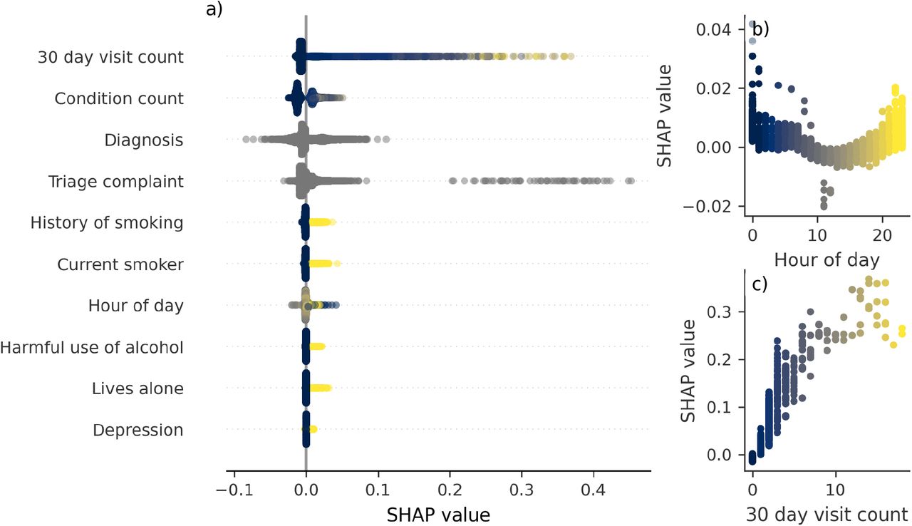
a) Plot summarizing the SHAP values for ten variables for each patient in the patient test set. They are ordered by the global impact the feature has on the explanation (practically, equal to the mean absolute SHAP value of the feature across all attendances). For the binary variables (i.e., the condition indicators) this favours variables with a high number of occurrences (i.e., more common conditions), not necessarily those which have the highest reattendance risk. b) SHAP value against recorded hour of day for time of registration for a given attendance (dots). c) SHAP value against number of emergency department visits in the 30 days prior to the given attendance (dots). In panels b and c vertical dispersion is the result of interaction with other variables in the feature set. All panels are coloured by the magnitude of the respective variable for the given data point, with lighter colours indicating higher values (e.g., inspect panels b and c). Grey data points correspond to non-binary categorical variables.
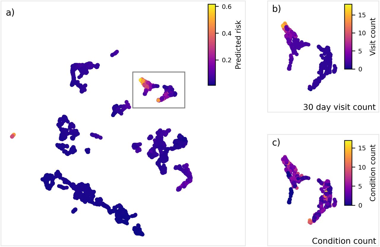
We then project the explanations for all attendances into a lower-dimensional (2D) ‘explanation’ space using the UMAP algorithm (see Methods for details), this projection provides insight into the different high-level groups of explanations provided by our model. The two-dimensional embedding of the attendances in the patient hold-out test set into the explanation space is visualised in Figure 4a. Attendances close in this space share more similar explanations for their predicted reattendance risk and we can see clear regions (colour) in the explanation space associated with increased reattendance risk. In Figures 5 b and c we display the attendances within the solid grey box, but now coloured by the number of visits in the 30 days preceding the given attendance the patient made to the emergency department and the number of medical conditions recorded in their electronic health record. Overall, this region highlights patients who are frequent attenders (number of visits in the 30 days preceding the attendance equal to 1 or more) and is separated into two sub regions: patients with a high attendance frequency (the left group in Figure 4b) and those who have attended once in the last 30-days and have at least one previous medical condition (the right group in Figure 4b).
a) All attendances in the patient hold-out test set visualised in the explanation space, colour indicates the predicted reattendance risk for the respective attendance. Coloured rectangles highlight regions of interest. The solid grey line indicates the region of interest plotted in panels b and c. b) Attendances within the solid grey region of interest in panel a, coloured by the patient’s 30-day visit count at the given attendance. c) Attendances within the solid grey region of interest in panel a, coloured by the patient’s condition count at the given attendance. This embedding was created by clustering the prediction explanations (generated using the TreeExplainer algorithm) for each emergency department attendance using the UMAP algorithm. Generally, closer data points share a more similar explanation for their predicted reattendance risk.
Discussion
Our final 72-hour reattendance risk model achieved an AUROC of 0.748 and an average precision of 0.250 on a set of attendances independent to the training set. Qualitatively, our model can use a patient’s (local) medical history and attendance level information to predict their reattendance risk with moderate performance. In parallel, we trained an explanation model, which can explain the model’s predictions at an attendance level (Figure 3 and Supplementary Figure 6) level. We projected the explanations into a two-dimensional space (Figure 4), with instances sharing similar explanations being closer in this space. Such a visualisation can be used as a tool to understand the different sub-groups at risk of reattendance, which could be used by the clinical care team to design interventions based on where a given attendance resides within the explanation space, ultimately facilitating the deployment of the machine-learnt model in a more informed manner.
Our final model (model p in Table 2) excluded two variables, pain score and measurements of vital signs. This was because while they were shown to be weakly predictive of reattendance risk in isolation (Table 2) they did not improve CV performance, despite increasing the model complexity, when included in models with larger numbers of variables, suggesting they are correlated to other features in the dataset. High correlation between variables is expected for clinical data, for example, one expects patient age, arrival mode, and vital signs all to latently encode the patient’s frailty, which is known to be related to a patients reattendance risk23.
Interestingly, our model’s validation performance increased when the model made use of the hour of day the attendance occurred (Supplementary Table 2). In our exploratory analysis, we found that the hour of day the attendance began displays clear correlation to the reattendance rate, with higher reattendance rates observed during the night (Supplementary Figure 3). By evaluating the observed SHAP values for the hour of day (Figure 3b) we can observe that our model has learned this trend, associating attendance registration during the night with a slightly higher (between zero and two percent) reattendance risk.
This trend could have several different origins. Firstly, we have found that the hour of day displays correlation with the reason for attendance with complaints associated with a higher risk of 72-hour reattendance more likely to present during the night alongside complaints associated with a lower risk of 72-hour reattendance less likely to present during the night. Secondly, it is reasonable that the staff fatigue and lower staffing levels could contribute to the increased reattendance for attendances occurring during the night, although we have no way of testing this hypothesis in our dataset.
Our model also makes use of ICD10 coded condition (e.g., type 1 diabetes, lives alone) indicators extracted from a patients electronic health record. These variables allow the model to identify medical conditions, comorbidities, and risks which are associated with increased reattendance risk and enables models to achieve moderate predictive performance (Table 2). Excluding the medical condition indicators and variables describing the reason for the attendance, the most important feature is the 30-day visit count which in part reflects the disproportionate use of EDs by frequent users24. In the visualisation of the attendances in the patient hold-out test set in the two-dimensional explanation space (Figure 4a), these frequent attenders (30 day visit count of two or more) are clearly segregated (solid grey rectangle in Figure 4a). Patients within this rectangle have a high chief triage complaint incidence of mental illness (7.5 % compared to average of 2.5 % for those not in this region), overdoses (5.6 % compared to 2.2 % for those not in this region), and abdominal pain (10.6 % compared to 7.7 % for those not in this region). This observation outlines how interventions can be designed based on explanation similarity as displayed in Figure 4. For example, while attendances within the solid grey box (i.e., frequent attenders) may benefit from support in the community to mitigate their reattendance risk, this will not necessarily be appropriate patients with a heighted reattendance risk but are suffering from an acute injury, associated with increased reattendance risk.
From a clinical perspective it is important to investigate the subset of reattendances which are also readmissions (i.e., reattendances to the emergency department which result in the patient being admitted). In these cases, there is increased risk that there was missed critical illness or injury at the initial attendance, and they are important to evaluate for clinical assurance purposes. Overall, 37.1 % of reattendances end in readmission, resulting in a 72-hour readmission rate of 2.0 %. Evaluating our model’s predictions now with a target equal to whether the patient was readmitted within 72 hours we again evaluate our model and find it has an AUROC of 0.804 and an average precision of 0.087 on the hold-out patient test set. The high AUROC means the model displays high discernibility between attendances which result in readmission and those that do not. The low average precision reflects that readmissions only make up a minority fraction of reattendances and the false positive rate increases as a result of the large class imbalance. Overall, these results demonstrate our classifier can identify the subset of reattendances which are also readmissions with a similar predictive performance as reattendances which do not result in admission – a particularly important result since these two different outcomes will likely merit different interventional strategies to reduce the risk of reattendance/readmission.
A limitation of our study, shared with other investigations of machine-learning use in EDs25, is that its primary data source is the structured past medical history, which is unavailable for many patients. This could lead to our model discriminating against people without a clinical history at the emergency department and associated hospital. We mitigate this through the use of visit-level information and this bias can be further reduced by linking to community datasets (e.g., GP records) to get a view of patient comorbidities. However, in a deployment scenario this bias could be minimized further by using the model as an alert tool – its results only being displayed for patients it predicts to be at high risk of reattendance and otherwise will be entirely invisible to clinical staff who would be free to carry out standard clinical practice in cases where the alarm is not raised.
Practically, since the model uses only information available to clinicians at the time of the emergency department visit the model has a relatively low barrier to implementation. Despite this, it will be essential to perform prospective, randomized clinical trials of any implementation, investigating the efficacy of these predictive risk models, the associated interventions prospectively and, importantly, analysing how they impact decision making. Ultimately, deployment of a machine-learning model could eventually invalidate the model by changing the behaviours and descriptors of reattendances by altering the clinical decision made. In the short term, a relatively low-risk implementation of a machine-learnt model trained to identify patients at risk of reattendance would be in the implementation of a low-recall and high-precision alert system (for example, the configuration presented in Figure 2c). This would only raise alarms for the cases the model believes are at the highest risk and suggest appropiate clinically-validated intervention or additional clinical review. On average, using the configuration displayed in Figure 2c, this would have raised an alarm for only 1.5 % of attendances in which a decision to discharge was made (approximately 2 times per day) and would expect to be correct approximately 50 % of the time – mitigating the risk of alarm fatigue and maintaining confidence in the model because of its modest precision, albeit with a limited impact because of the models low recall. As model performance improves, this configuration could be re-evaluated and changed to increase the impact of the model.
When considering deployment it is important to discuss the context in which these predictive models could be prospectively deployed. Our model was trained and retrospectively evaluated using data obtained local to the emergency department in Southampton, using data available to clinicians during standard clinical practice. This is clearly an advantage if the model is to be used at this location – the biases in the data and attendance characteristics will likely reflect what the model will encounter in production. Conversely, this does mean that the model will not necessarily generalize to different EDs without first training on their local data, this will be particularily prominient in EDs with a catchment zone with very different demographics to Southampton, which would have a differing disease prevalence and characteristics at presentation to the emergency department. Despite this, since our model contains variables either in the standard UK emergency care dataset or regularily available to EDs nationally, it is possible to evaluate this model directly in other EDs with little alteration. External validation of our model using data from different EDs is essential before prospective deployment beyond the department at which the training data was sourced.
Conclusion
In conclusion, we have constructed and retrospectively evaluated a gradient boosted decision tree classifier capable of predicting the 72-hour reattendance risk for a patient at the point of discharge from an emergency department. The highest performing model achieved an AUROC of 0.748 and an average precision of 0.250 on a set of attendances independent to the training set. We investigated the variables most indicative of risk and showed these were patient level factors (medical history) rather than visit level variables such as recorded vital signs. We demonstrated how explainable machine learning can be used to investigate the decisions a model is making and that they could potentially be used to inform intervention design. We suggested an implementation of the algorithm in a low-recall high-precision configuration such that alarms are only raised if the model deems the patient to be at a (clinically defined) heighted risk of reattendance. External validation and prospective clinical trials of these models are essential, with considerable consideration given to the planned intervention resulting from the model’s recommendation and the impact this would have on clinical decisions.
Data Availability
The data that support the findings of this study are available from UHS, but restrictions apply to the availability of these data, which were used under license for the current study, and so are not publicly available. Data are however available from the authors upon reasonable request and with permission of UHS.
Author contributions statement
FPC performed the data analysis and modelling. DKB and ZDZ discussed and commented on the analysis with FPC. NW and FPC obtained governance and ethical approval. MA and FB created the data extract. FPC, MJB and NW managed the study at the UoS. MK managed the study at UHS. FPC and MK designed the study with assistance from TWVD. MK and TWVD provided clinical guidance and insight. FPC wrote the first draft of the manuscript with assistance from MK and TWVD. All authors frequently discussed the work and commented and contributed to future drafts of the manuscript.
Additional information
Competing interests
The authors declare no competing interests.
Data Governance and ethics
This work received ethics approval from the University of Southampton’s Faculty of Engineering and Physical Science Research Ethics Committee (ERGO/FEPS/53164). Approval was also obtained from the NHS Health Research authority (20/HRA/1102, IRAS project ID 275577).
Data availability
The data that support the findings of this study are available from UHS, but restrictions apply to the availability of these data, which were used under license for the current study, and so are not publicly available. Data are however available from the authors upon reasonable request and with permission of UHS.
Acknowledgements
This work was supported by The Alan Turing Institute under the EPSRC grant EP/N510129/1. We acknowledge support from the NIHR Wessex ARC.
Footnotes
↵* F.P.Chmiel{at}soton.ac.uk
References


